

Intro
This article on the Pandas assign method is the first in a series of Professional Pandas blog posts that we will put out over the coming months. The goal of this series is to teach best practices about writing professional-grade pandas code. If you have questions or topics that you would like to dive into, please reach out on Twitter to @ponderdata or @__mharrison__, and if you’d like to see the notebook version of this blogpost, you can find it on Github here.
Try Ponder Today
Start running pandas and NumPy in your database within minutes!
In my opinion, one of the most underutilized methods in Pandas is the.assignmethod. My take (which may be extreme) is that.assignis the one true way to create a new column or update an existing column.
For those who don't want to read the whole article, here are my reasons for preferring .assign:
- You get around the dreaded
SettingWithCopyWarning - It enables chaining
- It forces you to write readable code that you, your future self, and your colleagues will appreciate
- It eases otherwise difficult operations
I get that this "only use .assign" may be extreme, but I encourage you to try it out first before you knock it. If you still hate it after trying it out, please send me your before and after code, because I am curious what happened.
For those still reading, let’s jump in!
Load data
To explore uses of the Pandas assign method, I'm going to use a dataset of meteorological data from a ski resort called Alta.
This data set has some descriptive columns and some daily facts:
- PRCP – liquid precipitation (inches)
- SNOW – snowfall (inches)
- SNWD – snow on the ground (inches)
- TMAX – maximum temperature (F)
- TMIN – minimum temperature (F)
- TOBS – temperature (F) at observation time
Let's load the data and create a tweak_alta function to pull out the columns we want.
In [1]:import modin.pandas as pd
raw = pd.read_csv('https://github.com/mattharrison/datasets/raw/master'
'/data/alta-noaa-1980-2019.csv', parse_dates=['DATE'])
def tweak_alta(df):
return (df
.loc[:, ['STATION', 'NAME', 'LATITUDE', 'LONGITUDE', 'ELEVATION', 'DATE',
'PRCP', 'SNOW', 'SNWD', 'TMAX', 'TMIN', 'TOBS']]
)
alta = tweak_alta(raw)
alta
Out [1]:STATION NAME LATITUDE LONGITUDE ELEVATION DATE PRCP SNOW SNWD TMAX TMIN TOBS
0 USC00420072 ALTA, UT US 40.5905 -111.6369 2660.9 1980-01-01 0.10 2.0 29.0 38.0 25.0 25.0
1 USC00420072 ALTA, UT US 40.5905 -111.6369 2660.9 1980-01-02 0.43 3.0 34.0 27.0 18.0 18.0
2 USC00420072 ALTA, UT US 40.5905 -111.6369 2660.9 1980-01-03 0.09 1.0 30.0 27.0 12.0 18.0
3 USC00420072 ALTA, UT US 40.5905 -111.6369 2660.9 1980-01-04 0.00 0.0 30.0 31.0 18.0 27.0
4 USC00420072 ALTA, UT US 40.5905 -111.6369 2660.9 1980-01-05 0.00 0.0 30.0 34.0 26.0 34.0
... ... ... ... ... ... ... ... ... ... ... ... ...
14155 USC00420072 ALTA, UT US 40.5905 -111.6369 2660.9 2019-09-03 0.01 0.0 0.0 74.0 57.0 73.0
14156 USC00420072 ALTA, UT US 40.5905 -111.6369 2660.9 2019-09-04 0.00 0.0 0.0 77.0 52.0 74.0
14157 USC00420072 ALTA, UT US 40.5905 -111.6369 2660.9 2019-09-05 0.00 0.0 0.0 76.0 54.0 65.0
14158 USC00420072 ALTA, UT US 40.5905 -111.6369 2660.9 2019-09-06 0.07 0.0 0.0 66.0 52.0 60.0
14159 USC00420072 ALTA, UT US 40.5905 -111.6369 2660.9 2019-09-07 0.00 0.0 0.0 68.0 45.0 64.0
14160 rows x 12 columns(Notice that we are using the Modin library above,import modin.pandas as pd. However, this same code will run with the Pandas library by only changing that line toimport pandas as pd.)
Create a new column
A common operation is adding a column to a dataframe.
Most create a column by using index assignment. This is convenient because:
- It looks like a dictionary operation that Python users are used to
- It (usually) overwrites the data making it a low overhead operation
There are also some disadvantages:
- It might cause a
SettingWithCopyWarning - It does not return a dataframe. Hence it cannot be used in a chain of operations
- Many users create intermediate variables (and call
.copyon the dataframe), thus removing the low overhead benefit
Below I will create a copy of the dataframe, alta_bad, and add a new column, PRCP_CM, that stores daily precipitation measured in centimeters. This is how many folks add columns to dataframes:
In [2]:alta_bad = alta.copy()
alta_bad['PRCP_CM'] = alta_bad.PRCP * 2.54Using Pandas assign instead
I prefer using the .assign method to create new columns. It also has some advantages and disadvantages. The advantages are:
- It returns a new dataframe so you can chain operations
- It sidesteps the
SettingWithCopyWarningcompletely. (As in, you will NEVER see it or deal with it). - It makes your code read like a recipe
- It forces you to think about the order of column creation for dependent columns
- It allows you to create multiple columns
- It lets you merge in a dataframe
The disadvantages of using the .assign method in Pandas:
- It copies the dataframe (in the Pandas implementation)
- Because it uses keyword parameters, you are limited to column names that are valid Python parameter names (unless you do
**unpacking with a dictionary that has the column stored as a key) - It requires knowledge of
lambda functions if you want to work on intermediate dataframes
Here is how I would add the PRCP_CM column using .assign:
In [3]:(alta
.assign(PRCP_CM=alta.PRCP * 2.54)
)
Out [3]: STATION NAME LATITUDE LONGITUDE ELEVATION DATE PRCP SNOW SNWD TMAX TMIN TOBS PRCP_CM
0 USC00420072 ALTA, UT US 40.5905 -111.6369 2660.9 1980-01-01 0.10 2.0 29.0 38.0 25.0 25.0 0.2540
1 USC00420072 ALTA, UT US 40.5905 -111.6369 2660.9 1980-01-02 0.43 3.0 34.0 27.0 18.0 18.0 1.0922
2 USC00420072 ALTA, UT US 40.5905 -111.6369 2660.9 1980-01-03 0.09 1.0 30.0 27.0 12.0 18.0 0.2286
3 USC00420072 ALTA, UT US 40.5905 -111.6369 2660.9 1980-01-04 0.00 0.0 30.0 31.0 18.0 27.0 0.0000
4 USC00420072 ALTA, UT US 40.5905 -111.6369 2660.9 1980-01-05 0.00 0.0 30.0 34.0 26.0 34.0 0.0000
... ... ... ... ... ... ... ... ... ... ... ... ... ...
14155 USC00420072 ALTA, UT US 40.5905 -111.6369 2660.9 2019-09-03 0.01 0.0 0.0 74.0 57.0 73.0 0.0254
14156 USC00420072 ALTA, UT US 40.5905 -111.6369 2660.9 2019-09-04 0.00 0.0 0.0 77.0 52.0 74.0 0.0000
14157 USC00420072 ALTA, UT US 40.5905 -111.6369 2660.9 2019-09-05 0.00 0.0 0.0 76.0 54.0 65.0 0.0000
14158 USC00420072 ALTA, UT US 40.5905 -111.6369 2660.9 2019-09-06 0.07 0.0 0.0 66.0 52.0 60.0 0.1778
14159 USC00420072 ALTA, UT US 40.5905 -111.6369 2660.9 2019-09-07 0.00 0.0 0.0 68.0 45.0 64.0 0.0000
14160 rows x 13 columnsChaining interlude
Let's take a break from discussing the .assign method for a moment.
This section might be controversial. My advice is to hold back your cringe reflex and hear me out. (Also, I would advise you to try out this style on your own code. My experience is that many who initially are repulsed by this have a wonderful epiphany when they try it, and it completely changes the way they write Pandas code.)
Folks who read my book, Effective Pandas, or follow my Pandas content know that I’m a big proponent of chaining.
What is chaining?
Chaining is writing a series of operations to a dataframe to manipulate it. Each operation works on the result of the previous operation.
One complaint I have against the many “learn to use Pandas” blog posts scattered about the internet is that they teach a method in isolation. In practice, you almost never perform an operation to data in isolation. There are multiple operations that are required to change column types, update values, deal with missing data, aggregate, plot, etc. But generally, you only care about the end result. The intermediate data along the way is not important.
Let’s assume that you wanted to summarize the Alta data by week. You might:
- Filter out columns
- Group by the date
- Aggregate different columns (by different functions)
- Create a new column with the NAME of the ski resort
- Create a new column with the weekly range
Let’s also assume that the resort was named “Alta Ski Resort” before year 2000 and just “Alta” after.
Most folks would write code like this:
In [4]:my_cols = ['STATION', 'NAME', 'LATITUDE', 'LONGITUDE', 'ELEVATION', 'DATE',
'PRCP', 'SNOW', 'SNWD', 'TMAX', 'TMIN', 'TOBS']
df1 = alta[my_cols]
grouped_df = df1.groupby(pd.Grouper(key='DATE', freq='W'))
df2 = grouped_df.agg({'PRCP': 'sum', 'TMAX': 'max', 'TMIN': 'min',
'SNOW': 'sum', 'SNWD': 'mean'})
df3 = df2.reset_index()
df3[df3.DATE < '2000']['LOCATION'] = 'Alta Ski Resort'
df3[df3.DATE >= '2000']['LOCATION'] = 'Alta'
df3['T_RANGE'] = df3.TMAX - df3.TMIN
df3
Out [4]:DATE PRCP TMAX TMIN SNOW SNWD T_RANGE
0 1980-01-06 0.68 42.0 12.0 7.0 30.500000 30.0
1 1980-01-13 8.76 33.0 -5.0 63.0 48.142857 38.0
2 1980-01-20 4.68 40.0 15.0 34.0 63.285714 25.0
3 1980-01-27 0.00 43.0 10.0 0.0 57.000000 33.0
4 1980-02-03 2.58 38.0 -6.0 40.0 70.571429 44.0
... ... ... ... ... ... ... ...
2066 2019-08-11 1.09 78.0 42.0 0.0 0.000000 36.0
2067 2019-08-18 0.00 75.0 42.0 0.0 0.000000 33.0
2068 2019-08-25 0.00 76.0 45.0 0.0 0.000000 31.0
2069 2019-09-01 0.02 78.0 41.0 0.0 0.000000 37.0
2070 2019-09-08 0.08 78.0 45.0 0.0 0.000000 33.0
2071 rows × 7 columnsThey would find that the lines:
df3[df3.DATE < '2000']['LOCATION'] = 'Alta Ski Resort'
df3[df3.DATE >= '2000']['LOCATION'] = 'Alta'don’t really work and would probably change them to this (after searching around on the internet):
In [5]:df3.loc[df3.DATE < '2000','LOCATION'] = 'Alta Ski Resort'
df3.loc[df3.DATE >= '2000','LOCATION'] = 'Alta'
df3
Out [5]:DATE PRCP TMAX TMIN SNOW SNWD LOCATION T_RANGE SEASON
0 1980-01-06 0.68 42.0 12.0 7.0 30.500000 Alta Ski Resort 30.0 Ski 1979
1 1980-01-13 8.76 33.0 -5.0 63.0 48.142857 Alta Ski Resort 38.0 Ski 1979
2 1980-01-20 4.68 40.0 15.0 34.0 63.285714 Alta Ski Resort 25.0 Ski 1979
3 1980-01-27 0.00 43.0 10.0 0.0 57.000000 Alta Ski Resort 33.0 Ski 1979
4 1980-02-03 2.58 38.0 -6.0 40.0 70.571429 Alta Ski Resort 44.0 Ski 1979
... ... ... ... ... ... ... ... ... ...
2066 2019-08-11 1.09 78.0 42.0 0.0 0.000000 Alta 36.0 Summer 2019
2067 2019-08-18 0.00 75.0 42.0 0.0 0.000000 Alta 33.0 Summer 2019
2068 2019-08-25 0.00 76.0 45.0 0.0 0.000000 Alta 31.0 Summer 2019
2069 2019-09-01 0.02 78.0 41.0 0.0 0.000000 Alta 37.0 Summer 2019
2070 2019-09-08 0.08 78.0 45.0 0.0 0.000000 Alta 33.0 Summer 2019
2071 rows × 9 columnsNow let’s add a ski season to the rows. Generally a ski season starts in November and ends in April.
In [6]:df3['SEASON'] = 'Summer'
df3.loc[(df3.DATE.dt.month <= 4)
|(df3.DATE.dt.month >= 11), 'SEASON'] = 'Ski'
df3
Out [6]:DATE PRCP TMAX TMIN SNOW SNWD LOCATION T_RANGE SEASON
0 1980-01-06 0.68 42.0 12.0 7.0 30.500000 Alta Ski Resort 30.0 Ski
1 1980-01-13 8.76 33.0 -5.0 63.0 48.142857 Alta Ski Resort 38.0 Ski
2 1980-01-20 4.68 40.0 15.0 34.0 63.285714 Alta Ski Resort 25.0 Ski
3 1980-01-27 0.00 43.0 10.0 0.0 57.000000 Alta Ski Resort 33.0 Ski
4 1980-02-03 2.58 38.0 -6.0 40.0 70.571429 Alta Ski Resort 44.0 Ski
... ... ... ... ... ... ... ... ... ...
2066 2019-08-11 1.09 78.0 42.0 0.0 0.000000 Alta 36.0 Summer
2067 2019-08-18 0.00 75.0 42.0 0.0 0.000000 Alta 33.0 Summer
2068 2019-08-25 0.00 76.0 45.0 0.0 0.000000 Alta 31.0 Summer
2069 2019-09-01 0.02 78.0 41.0 0.0 0.000000 Alta 37.0 Summer
2070 2019-09-08 0.08 78.0 45.0 0.0 0.000000 Alta 33.0 Summer
2071 rows × 9 columnsFinally, let’s add a year to the SEASON:
In [7]:df3['SEASON'] = df3.SEASON + ' ' \
+ df3.DATE.dt.year.astype(str).where(df3.DATE.dt.month > 4,
(df3.DATE.dt.year - 1).astype(str))
df3
Out [7]:DATE PRCP TMAX TMIN SNOW SNWD LOCATION T_RANGE SEASON
0 1980-01-06 0.68 42.0 12.0 7.0 30.500000 Alta Ski Resort 30.0 Ski 1979
1 1980-01-13 8.76 33.0 -5.0 63.0 48.142857 Alta Ski Resort 38.0 Ski 1979
2 1980-01-20 4.68 40.0 15.0 34.0 63.285714 Alta Ski Resort 25.0 Ski 1979
3 1980-01-27 0.00 43.0 10.0 0.0 57.000000 Alta Ski Resort 33.0 Ski 1979
4 1980-02-03 2.58 38.0 -6.0 40.0 70.571429 Alta Ski Resort 44.0 Ski 1979
... ... ... ... ... ... ... ... ... ...
2066 2019-08-11 1.09 78.0 42.0 0.0 0.000000 Alta 36.0 Summer 2019
2067 2019-08-18 0.00 75.0 42.0 0.0 0.000000 Alta 33.0 Summer 2019
2068 2019-08-25 0.00 76.0 45.0 0.0 0.000000 Alta 31.0 Summer 2019
2069 2019-09-01 0.02 78.0 41.0 0.0 0.000000 Alta 37.0 Summer 2019
2070 2019-09-08 0.08 78.0 45.0 0.0 0.000000 Alta 33.0 Summer 2019
2071 rows × 9 columnsThis looks ok, and you have probably seen code like this. You’ve probably written code like this if you are reading this post.
It does have some issues. It spans multiple cells, creates unneeded intermediate variables, and might be buggy (note that the LOCATION column initially failed silently).
Let's use the Pandas .assign method and chaining to write it a little differently.
In [8]:def monthly_summary(df):
my_cols = ['STATION', 'NAME', 'LATITUDE', 'LONGITUDE', 'ELEVATION', 'DATE',
'PRCP', 'SNOW', 'SNWD', 'TMAX', 'TMIN', 'TOBS']
return (df
[my_cols]
.groupby(pd.Grouper(key='DATE', freq='W'))
.agg({'PRCP': 'sum', 'TMAX': 'max', 'TMIN': 'min', 'SNOW': 'sum', 'SNWD': 'mean'})
.reset_index()
.assign(LOCATION='Alta',
SEASON='Ski')
.assign(LOCATION=lambda df_: df_.LOCATION.where(
df_.DATE.dt.year >= 2000
,'Alta Ski Resort'),
T_RANGE=lambda df_: df_.TMAX - df_.TMIN,
SEASON=lambda df_:(df_
.SEASON
.where(
(df_.DATE.dt.month <= 4) | (df_.DATE.dt.month >= 11), 'Summer')
.add(' ')
.add(df_
.DATE.dt.year.astype(str)
.where(df_.DATE.dt.month > 4,
(df_.DATE.dt.year - 1).astype(str))))
)
)
monthly_summary(alta)
Out [8]:DATE PRCP TMAX TMIN SNOW SNWD LOCATION SEASON T_RANGE
0 1980-01-06 0.68 42.0 12.0 7.0 30.500000 Alta Ski Resort Ski 1979 30.0
1 1980-01-13 8.76 33.0 -5.0 63.0 48.142857 Alta Ski Resort Ski 1979 38.0
2 1980-01-20 4.68 40.0 15.0 34.0 63.285714 Alta Ski Resort Ski 1979 25.0
3 1980-01-27 0.00 43.0 10.0 0.0 57.000000 Alta Ski Resort Ski 1979 33.0
4 1980-02-03 2.58 38.0 -6.0 40.0 70.571429 Alta Ski Resort Ski 1979 44.0
... ... ... ... ... ... ... ... ... ...
2066 2019-08-11 1.09 78.0 42.0 0.0 0.000000 Alta Summer 2019 36.0
2067 2019-08-18 0.00 75.0 42.0 0.0 0.000000 Alta Summer 2019 33.0
2068 2019-08-25 0.00 76.0 45.0 0.0 0.000000 Alta Summer 2019 31.0
2069 2019-09-01 0.02 78.0 41.0 0.0 0.000000 Alta Summer 2019 37.0
2070 2019-09-08 0.08 78.0 45.0 0.0 0.000000 Alta Summer 2019 33.0
2071 rows × 9 columnsA false positive issue
One common comment that I hear when folks see code that looks like monthly_summary is: "This code must be hard to debug."
I beg to differ. It is written as a chain. But I didn’t write out all the code at once. I wrote one operation at a time. Then I ran the code and validated (debugged) that it was doing what I wanted.
There are a few pleasant aspects of code written this way. First, it is encapsulated in a function. This makes it easy to pull out into a script and use elsewhere. Also, because it is a function, there aren't any intermediate variables hanging around messing up the global namespace. For example, the my_cols variable is garbage collected when the function has finished executing.
Also, this chain reads like a recipe of steps:
- Pull out the columns
- Groupby by the date with a weekly (
'W') frequency - Aggregate the columns as indicated
- Push the index (the week date) into a column
- Add a temperature range (T_RANGE) column
- Add columns for LOCATION and SEASON
- Update the LOCATION and SEASON columns with logic
In fact, writing chains forces you to think about each step that you will perform on the data. It is a constraint that I find allows me to write better code. (Again, you might think I’m spewing crazy talk. Try it out and see how it helps with your code.)
This code is also easy to execute. It is all in one place. Another struggle with notebooks is cells strewn with data manipulation logic (that can be executed in arbitrary order). With the chained code, you can come back to this notebook in the future and run this cell with confidence, knowing that you weren’t missing running other random cells from the notebook.
Debugging this code is easy as well. I'm not going to dive into that here as I have devoted a whole chapter to that in my book, Effective Pandas (maybe I will do a future blog post on debugging if there is interest). In short, you can comment out the operations to see previous intermediate results or combine a.pipecall with abreakpoint()to jump into the debugger if you really want to.
Real issues with Pandas assign
Everything is not peaches and cream with the .assign method. There are some real issues with this code. One is that it requires understanding lambda expressions.
However, I think if you want to be a serious user of Pandas, it pays off to take a few minutes to understand lambda functions.
We use lambda expressions to create anonymous functions. These are just functions that we can inline in a call. In fact, we don’t really need to use them. We can define a normal function instead. I could write the line:
.assign(T_RANGE=lambda df_: df_.TMAX - df_.TMIN,As
.assign(T_RANGE=calc_range,If I had a calc_range function defined as:
def calc_range(df_):
    return df_.TMAX - df_.TMIN,
(Note I use the variabledf_ inmylambdato distinguish it fromdfthat was passed into themonthly_summaryfunction.)
Using alambdafunction (or a normal function) with.assignpasses in the current state of the dataframe into the function. Because we have aggregated the daily data to a weekly level, we can only calculate the weekly range from the current data and not the original daily data,df.
The lambda accepts the current state of the dataframe and should return a scalar value or a series to use for the new or updated column values.
The lines:
            .assign(...
                    LOCATION='Alta',
                    SEASON='Ski')
Create columns for LOCATION and SEASON with a single value. You can also set them to a series as well. They don't need lambdas because we are not dependent on the current state of the dataframe.
Another "issue" with Pandas assign is that we need a new call to it if we want to update a column again (like we do with LOCATION and SEASON). (Because .assign is leveraging named parameters in Python, we can't have two parameters with the same name).
Complaints that this code is “complicated” are valid, in my opinion. But the complication comes from Pandas’ lack of providing a clean interface for if else logic, not from the chain.
(I personally find the.wheremethod lacking and wish that Pandas had something similar to NumPy'sselectfunction for implementing conditional logic.)
Further refactoring
To address the “complicated” nature of creating the LOCATION and SEASON columns, you might consider refactoring the logic to create these columns into a function:
In [9]:def monthly_summary(df):
def get_location(df_):
return (df_
.assign(LOCATION='Alta')
.LOCATION
.where(df_.DATE.dt.year >= 2000, 'Alta Ski Resort')
)
def get_season(df_):
return (df_
.assign(SEASON='Ski')
.SEASON
.where((df_.DATE.dt.month <= 4) | (df_.DATE.dt.month >= 11), 'Summer')
.add(' ')
.add(df_
.DATE.dt.year.astype(str)
.where(df_.DATE.dt.month > 4, (df_.DATE.dt.year - 1).astype(str)))
)
my_cols = ['STATION', 'NAME', 'LATITUDE', 'LONGITUDE', 'ELEVATION', 'DATE',
'PRCP', 'SNOW', 'SNWD', 'TMAX', 'TMIN', 'TOBS']
return (df
[my_cols]
.groupby(pd.Grouper(key='DATE', freq='W'))
.agg({'PRCP': 'sum', 'TMAX': 'max', 'TMIN': 'min', 'SNOW': 'sum', 'SNWD': 'mean'})
.reset_index()
.assign(T_RANGE=lambda df_: df_.TMAX - df_.TMIN,
LOCATION=get_location,
SEASON=get_season
)
)
monthly_summary(alta)
Out [9]:DATE PRCP TMAX TMIN SNOW SNWD T_RANGE LOCATION SEASON
0 1980-01-06 0.68 42.0 12.0 7.0 30.500000 30.0 Alta Ski Resort Ski 1979
1 1980-01-13 8.76 33.0 -5.0 63.0 48.142857 38.0 Alta Ski Resort Ski 1979
2 1980-01-20 4.68 40.0 15.0 34.0 63.285714 25.0 Alta Ski Resort Ski 1979
3 1980-01-27 0.00 43.0 10.0 0.0 57.000000 33.0 Alta Ski Resort Ski 1979
4 1980-02-03 2.58 38.0 -6.0 40.0 70.571429 44.0 Alta Ski Resort Ski 1979
... ... ... ... ... ... ... ... ... ...
2066 2019-08-11 1.09 78.0 42.0 0.0 0.000000 36.0 Alta Summer 2019
2067 2019-08-18 0.00 75.0 42.0 0.0 0.000000 33.0 Alta Summer 2019
2068 2019-08-25 0.00 76.0 45.0 0.0 0.000000 31.0 Alta Summer 2019
2069 2019-09-01 0.02 78.0 41.0 0.0 0.000000 37.0 Alta Summer 2019
2070 2019-09-08 0.08 78.0 45.0 0.0 0.000000 33.0 Alta Summer 2019
2071 rows × 9 columnsCreate a plot
Ok, a weekly summary is nice. But the goal of most manipulating data is not the individual step but creating a result that we can use to inspire, inform, or take action. Let’s use Matplotlib to create a plot of snow on the ground during a season.
This is similar to what is found in my book, Pandas Cookbook 1.x, and was inspired by a plot created by Trud Antzee (@Antzee_).
In [10]:import matplotlib.pyplot as plt
def plot_season(df, year, fig, ax):
blue = '#99ddee'
white = '#fff'
data = (df
.query(f'SEASON=="Ski {year}"')
)
for side in 'top,right,bottom,left'.split(','):
ax.spines[side].set_visible(False)
ax.tick_params(axis='both', colors=white)
ax.tick_params(axis='both', colors=white)
ax.tick_params(axis='x', which='minor', colors=white)
ax.fill_between(data.DATE, data.SNWD, color='white')
ax.set_facecolor(blue)
ax.set_ylim(0, 150)
ax.set_title(f'{year} Season Snowfall', fontsize=16, color=white)
def facet_plot(df, years):
blue = '#99ddee'
white = '#fff'
fig, axs = plt.subplots(ncols=2, nrows=(len(years)//2),
figsize=(16, 10), facecolor=blue)
axs = axs.flatten()
for i, year in enumerate(years):
plot_season(df, year, fig, axs[i])
fig.suptitle('Alta Snowfall (@__mharrison__)', fontsize=20, color=white)
fig.tight_layout()
return fig
_ = (monthly_summary(alta)
.pipe(facet_plot, years=['2000', '2005','2010', '2015'])
)
Out [10]: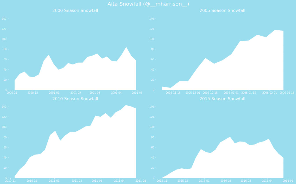
Final code
Thanks for getting this far. I hope you have a better understanding of using the .assign method. Also I hope you appreciate that operations do not occur in isolation.
We showed how to take "traditional" Pandas code, refactor it into chains and functions. I would love to hear your feedback. How are you going to use the Pandas assign method? Please share examples of applying chains like this to your code on Twitter, and tag @ponderdata and @__mharrison__ (and follow us on Twitter for more content like this). What insights did you have as you were doing it?
In [11]:import matplotlib.pyplot as plt
import modin.pandas as pd
raw = pd.read_csv('https://github.com/mattharrison/datasets/raw/master/data/alta-noaa-1980-2019.csv',
parse_dates=['DATE'])
def tweak_alta(df):
return (df
.loc[:, ['STATION', 'NAME', 'LATITUDE', 'LONGITUDE', 'ELEVATION', 'DATE',
'PRCP', 'SNOW', 'SNWD', 'TMAX', 'TMIN', 'TOBS']]
)
def monthly_summary(df):
def get_location(df_):
return (df_
.assign(LOCATION='Alta')
.LOCATION
.where(df_.DATE.dt.year >= 2000, 'Alta Ski Resort')
)
def get_season(df_):
return (df_
.assign(SEASON='Ski')
.SEASON
.where((df_.DATE.dt.month <= 4) | (df_.DATE.dt.month >= 11), 'Summer')
.add(' ')
.add(df_
.DATE.dt.year.astype(str)
.where(df_.DATE.dt.month > 4, (df_.DATE.dt.year - 1).astype(str)))
)
my_cols = ['STATION', 'NAME', 'LATITUDE', 'LONGITUDE', 'ELEVATION', 'DATE',
'PRCP', 'SNOW', 'SNWD', 'TMAX', 'TMIN', 'TOBS']
return (df
[my_cols]
.groupby(pd.Grouper(key='DATE', freq='W'))
.agg({'PRCP': 'sum', 'TMAX': 'max', 'TMIN': 'min', 'SNOW': 'sum', 'SNWD': 'mean'})
.reset_index()
.assign(T_RANGE=lambda df_: df_.TMAX - df_.TMIN,
LOCATION=get_location,
SEASON=get_season
)
)
def plot_season(df, year, fig, ax):
blue = '#99ddee'
white = '#fff'
data = (df
.query(f'SEASON=="Ski {year}"')
)
for side in 'top,right,bottom,left'.split(','):
ax.spines[side].set_visible(False)
ax.tick_params(axis='both', colors=white)
ax.tick_params(axis='both', colors=white)
ax.tick_params(axis='x', which='minor', colors=white)
ax.fill_between(data.DATE, data.SNWD, color='white')
ax.set_facecolor(blue)
ax.set_ylim(0, 150)
ax.set_title(f'{year} Season Snowfall', fontsize=16, color=white)
def facet_plot(df, years):
blue = '#99ddee'
white = '#fff'
fig, axs = plt.subplots(ncols=2, nrows=(len(years)//2),
figsize=(16, 10), facecolor=blue)
axs = axs.flatten()
for i, year in enumerate(years):
plot_season(df, year, fig, axs[i])
fig.suptitle('Alta Snowfall (@__mharrison__)', fontsize=20, color=white)
fig.tight_layout()
return fig
_ = (raw
.pipe(tweak_alta)
.pipe(monthly_summary)
.pipe(facet_plot, years=['2000', '2005','2010', '2015'])
)
Out [11]:Ponder
Ponder is the company that lets you run your Python data workflows (in Pandas or NumPy) securely, seamlessly, and scalably in your data warehouse or database. Sign up for a free trial!
Try Ponder Today
Start running your Python data science workflows in your database within minutes!