

TLDR: In this post, we compare Pandas vs. SQL on the third of three axes: convenience. We describe six ways in which the Pandas dataframe data model is more convenient for data science and machine learning use cases.
In this fourth offering of our epic battle between Pandas vs. SQL, we illustrate how Pandas is more convenient than SQL for data science and machine learning. Pandas was designed by data scientists for data scientists, and benefited from thousands of improvements contributed back enthusiastically by the open-source data science community — all with an eye towards greater utility and ease-of-use. So it’s no surprise that it’s a good fit!
Before we begin, if you missed our previous Pandas vs. SQL offerings, you can still catch up here: Part 1: The Food Court and the Michelin-Style Restaurant, Part 2: Pandas Is More Concise, and Part 3: Pandas Is More Flexible. Our previous posts focused on comparisons on the dataframe data model and dataframe algebra — in this post, we focus on the dataframe ergonomics: specifically, how dataframes are used.
For easy lookup, here is a handy list of the multiple ways Pandas dataframes are more convenient than their relational/SQL counterparts:
- In Pandas, you can incrementally construct queries as you go along; in SQL, you cannot.
- In Pandas, operating on and naming intermediate results is easy; in SQL it is harder.
- In Pandas, it is easy to get a quick sense of the data; in SQL it is much harder.
- Pandas has native support for visualization; SQL does not.
- Pandas makes it easy to do machine learning; SQL does not.
- Pandas preserves order to help users verify correctness of intermediate steps — and allows users to operate on order; SQL does not.
Or, you can skip ahead to the conclusion!
For this post, we’ll use a dataset from Kaggle’s 5 day data cleaning challenge; this is a dataset of building permits in San Francisco.
In [1]:sf_permits = pd.read_csv("building-permit-applications-data/Building_Permits.csv")
sf_permits.head()
Out [1]: Permit Number Permit Type Permit Type Definition Permit Creation Date Block Lot Street Number Street Number Suffix Street Name Street Suffix ... Neighborhoods - Analysis Boundaries Zipcode Location Record ID
0 201505065519 4 sign - erect 05/06/2015 0326 023 140 NaN Ellis St ... Tenderloin 94102.0 (37.785719256680785, -122.40852313194863) 1380611233945
1 201604195146 4 sign - erect 04/19/2016 0306 007 440 NaN Geary St ... Tenderloin 94102.0 (37.78733980600732, -122.41063199757738) 1420164406718
2 201605278609 3 additions alterations or repairs 05/27/2016 0595 203 1647 NaN Pacific Av ... Russian Hill 94109.0 (37.7946573324287, -122.42232562979227) 1424856504716
3 201611072166 8 otc alterations permit 11/07/2016 0156 011 1230 NaN Pacific Av ... Nob Hill 94109.0 (37.79595867909168, -122.41557405519474) 1443574295566
4 201611283529 6 demolitions 11/28/2016 0342 001 950 NaN Market St ... Tenderloin 94102.0 (37.78315261897309, -122.40950883997789) 144548169992
5 rows × 43 columns
1. In Pandas, you can incrementally construct queries as you go along; in SQL, you cannot.
An important distinction between Pandas and SQL is that Pandas allows users to incrementally layer operations on top of others to construct more complicated queries. At the same time, users can inspect intermediate results of these query fragments — in an effort to verify correctness as they go along. Debugging is a breeze with Pandas!
So in our dataset, say we want to focus on permits corresponding to Geary Street. We can extract that subset of the dataset as follows:
In [2]:sf_permits[sf_permits['Street Name'] == 'Geary']
Out [2]: Permit Number Permit Type Permit Type Definition Permit Creation Date Block Lot Street Number Street Number Suffix Street Name ... Neighborhoods - Analysis Boundaries Zipcode Location Record ID
1 201604195146 4 sign - erect 04/19/2016 0306 007 440 NaN Geary ... Tenderloin 94102.0 (37.78733980600732, -122.41063199757738) 1420164406718
51 M843007 8 otc alterations permit 10/12/2017 1095 005 2425 NaN Geary ... Lone Mountain/USF 94115.0 (37.78231492051284, -122.44311204170013) 148305089457
193 201708023634 1 new construction 08/02/2017 1094 001 2675 NaN Geary ... Lone Mountain/USF 94115.0 (37.781833472205996, -122.4457308481205) 147295789456
... ... ... ... ... ... ... ... ... ... ... ... ... ... ...
198883 M893427 8 otc alterations permit 02/23/2018 0315 021 377 NaN Geary ... Tenderloin 94102.0 (37.78696971667916, -122.40936701144197) 149834069380
1966 rows × 43 columns
One thing we might have noticed is that Geary spans many neighborhoods, encoded here as'Neighborhoods - Analysis Boundaries'. Suppose we only wanted to examine this column'Neighborhoods - Analysis Boundaries'(and drop the remaining 42 columns), we can simply append the clause[['Neighborhoods - Analysis Boundaries']]at the end of the previous expression.
In [3]:sf_permits[sf_permits['Street Name'] == 'Geary'][['Neighborhoods - Analysis Boundaries']]
Out [3]: Neighborhoods - Analysis Boundaries
65869 Financial District/South Beach
116244 Financial District/South Beach
116523 Financial District/South Beach
94565 Financial District/South Beach
20873 Financial District/South Beach
... ...
160946 NaN
160968 NaN
161383 NaN
165628 NaN
191848 NaN
1966 rows × 1 columns
This is a lot of rows: 1966. Then, as our last two steps, say we want to identify the neighborhoods on Geary with the most permits. One way to do so is by appending a'sort_values'followed by a'value_counts'.
In [4]:sf_permits[sf_permits['Street Name'] == 'Geary'][['Neighborhoods - Analysis Boundaries']].sort_values(by = ['Neighborhoods - Analysis Boundaries']).value_counts()
Out [4]: Neighborhoods - Analysis Boundaries
Tenderloin 581
Outer Richmond 384
Financial District/South Beach 268
Lone Mountain/USF 197
Inner Richmond 179
Presidio Heights 156
Japantown 134
Western Addition 37
dtype: int64
Interesting, so the top neighborhood is the Tenderloin, followed by Outer Richmond. Note that while this sequence of operations can certainly be expressed in SQL, it would have been much more painful. We can't simply append operators at the end of one's SQL query: there are specific locations within the query where we would need to make changes. For example, to change which columns are displayed we would need to modify the SELECT portion of the query early on. Pandas instead allows you to think operationally (or imperatively) — and construct your final result step-by-step, all the while examining intermediate results.
2. In Pandas, operating on and naming intermediate results is easy; in SQL it is harder.
Pandas, since it is embedded in a real programming language, Python, borrows many of the familiar programmatic idioms for operating on dataframes. In particular, we can assign a dataframe expression to a variable; these variables can then be operated on and/or assigned to other variables.
We’ll take a simple example to illustrate. Since this dataset is from a data cleaning challenge, say we suspect that there might be many null values. We can check how many there are per column, using the following:
In [5]:missing_values_count = sf_permits.isnull().sum()
missing_values_count
Out [5]:Permit Number 0
Permit Type 0
Permit Type Definition 0
Permit Creation Date 0
Block 0
Lot 0
Street Number 0
Street Number Suffix 196684
Street Name 0
Street Suffix 2768
Unit 169421
Unit Suffix 196939
Description 290
Current Status 0
Current Status Date 0
Filed Date 0
Issued Date 14940
Completed Date 101709
First Construction Document Date 14946
Structural Notification 191978
Number of Existing Stories 42784
Number of Proposed Stories 42868
Voluntary Soft-Story Retrofit 198865
Fire Only Permit 180073
Permit Expiration Date 51880
Estimated Cost 38066
Revised Cost 6066
Existing Use 41114
Existing Units 51538
Proposed Use 42439
Proposed Units 50911
Plansets 37309
TIDF Compliance 198898
Existing Construction Type 43366
Existing Construction Type Description 43366
Proposed Construction Type 43162
Proposed Construction Type Description 43162
Site Permit 193541
Supervisor District 1717
Neighborhoods - Analysis Boundaries 1725
Zipcode 1716
Location 1700
Record ID 0
dtype: int64
That’s a lot of null values! Suppose I want to create a cleaned version of my dataset, dropping columns with too many null values, with the threshold set at 190000 non-null values. (The overall dataset has about 199000 rows.)
In [6]:sf_permits_cleaned = sf_permits.dropna(axis='columns',thresh=190000)
sf_permits_cleaned
Out [6]: Permit Number Permit Type Permit Type Definition Permit Creation Date Block Lot Street Number Street Name Description Current Status Current Status Date Filed Date Record ID
0 201505065519 4 sign - erect 05/06/2015 0326 023 140 Ellis ground fl facade: to erect illuminated, electr... expired 12/21/2017 05/06/2015 1380611233945
1 201604195146 4 sign - erect 04/19/2016 0306 007 440 Geary remove (e) awning and associated signs. issued 08/03/2017 04/19/2016 1420164406718
... ... ... ... ... ... ... ... ... ... ... ... ... ...
198898 M863747 8 otc alterations permit 12/06/2017 0298 029 795 Sutter street space permit issued 12/06/2017 12/06/2017 1489608233656
198899 M864287 8 otc alterations permit 12/07/2017 0160 006 838 Pacific street space permit issued 12/07/2017 12/07/2017 1489796283803
198900 rows × 13 columns
Wow - the number of columns drops from 43 to just 13. As we saw here, we were able to easily define a new variable'sf_permits_cleaned'(just like we created the previous variable'missing_values_count'), using standard programmatic variable assignment and subsequently operate on it. This approach is natural for programmers. In SQL, one can accomplish a similar effect via views, but defining views and operating on them is less intuitive and more cumbersome.
3. In Pandas, it is easy to get a quick sense of the data; in SQL it is much harder.
Pandas offers quick ways to understand the data and metadata of a dataframe. We've already seen examples of this when we print a dataframe by simply using its variable name, or if we use the functions'head/tail()'. For convenience, to fit on a screen, certain rows and columns are hidden away with'...'to help users still get a high-level picture of the data.
If we want to inspect a summary of the columns and their types, one convenient function offered by Pandas is'info()', which lists the columns of the dataset, their types, and number of null values. We can use this function to inspect the dataframe we just created.
In [7]:sf_permits_cleaned.info()
Out [7]:<class 'pandas.core.frame.dataframe'="">
RangeIndex: 198900 entries, 0 to 198899
Data columns (total 13 columns):
# Column Non-Null Count Dtype
--- ------ -------------- -----
0 Permit Number 198900 non-null object
1 Permit Type 198900 non-null int64
2 Permit Type Definition 198900 non-null object
3 Permit Creation Date 198900 non-null object
4 Block 198900 non-null object
5 Lot 198900 non-null object
6 Street Number 198900 non-null int64
7 Street Name 198900 non-null object
8 Description 198610 non-null object
9 Current Status 198900 non-null object
10 Current Status Date 198900 non-null object
11 Filed Date 198900 non-null object
12 Record ID 198900 non-null int64
dtypes: int64(3), object(10)
memory usage: 19.7+ MB
So it looks like the only column still containing null values is the description column; all
other columns are fully filled in.
Another useful Pandas function, targeted at numerical columns, is 'describe()', which provides a convenient summary of these columns, with counts, means, standard deviations, and quantiles.
In [8]:sf_permits_cleaned.describe()
Out [8]: Permit Type Street Number Record ID
count 198900.000000 198900.000000 1.989000e+05
mean 7.522323 1121.728944 1.162048e+12
std 1.457451 1135.768948 4.918215e+11
min 1.000000 0.000000 1.293532e+10
25% 8.000000 235.000000 1.308567e+12
50% 8.000000 710.000000 1.371840e+12
75% 8.000000 1700.000000 1.435000e+12
max 8.000000 8400.000000 1.498342e+12
Hmm, so there appears to be a street number 0. Curious!
Unfortunately, SQL offers no similar conveniences to understand the shape and characteristics of one’s dataset — you’d have to write custom queries for this purpose. For the previous example, the length of this query would be proportional to the number of numeric columns.
4. Pandas has native support for visualization; SQL does not.
Analysis of tables of numbers will only get your so far. Often what you need are visual ways of making sense of information in dataframes. Unlike SQL, which requires you to load your data into a separate visualization or BI (Business Intelligence) tool, Pandas offers in-built visualization support right within the library. For example, I can simply call'plot()'to see a bar chart of the'Current Status'of various permits.
In [9]:sf_permits_cleaned["Current Status"].value_counts().plot(kind ="bar")
Out [9]: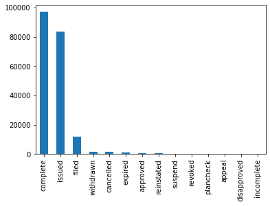
It looks like the vast majority of permits are in the completed, issued, and filed categories, with a small number in other categories.
The power of this feature is obvious: unlike SQL databases, you don’t need to leave the library if you want to generate visualizations — you can do it right there! If you’d like to “power-up” your visualization experience, there are any number of visualization libraries that integrate tightly with pandas, including Matplotlib, seaborn, and altair. And if you’re lazy, like me, and don’t wish to write any code at all to generate visualizations, you can use Lux, our Pandas-native visualization recommendation library, to generate visualizations for you automatically, all tuned to your dataset. Read more about Lux here.
5. Pandas makes it easy to do machine learning; SQL does not.
Machine learning is a key component of data science, enabling users to not just make sense of unstructured data such as images, video, and text, but also make predictions about the future. Since Pandas is tightly integrated into the data science ecosystem, it comes as no surprise that it works well with machine learning libraries, including common ones like scikit-learn, pytorch, numpy, among others. Here, we’ll use the spaCy library, a relatively new natural language processing library, to make sense of a text column in our dataset. SpaCy offers various word pretrained models to perform word embedding, named entity recognition, part of speech tagging, classification, among others. To install spaCy, we run the following commands:
In [10]:!pip install -U spacy
!python -m spacy download en_core_web_md
Now that we've installed it, suppose we want to understand the type of activities (e.g., demolition, removal, replacement, etc.) involved in each permit application (i.e. row) in our dataset. This is hard to understand upfront, but is buried within the text field,'Description'. Let's use the package to extract a list of verbs that are mentioned in this field. As part of this, we first load spaCy's'en_core_web_md'model, and then follow it up by extracting each verb in the tokenization of the description using the model, storing it in an array, as follows.
In [11]:import spacy
nlp = spacy.load("en_core_web_md")
descriptions = sf_permits_cleaned[["Permit Number", "Description"]]
descriptions["Verbs"] = descriptions.apply(lambda x: [y.lemma_ for y in nlp(x["Description"].astype(str)) if y.pos_=="VERB"], axis = 1)
descriptions.head()
Out [11]: Permit Number Description Entities
0 201505065519 ground fl facade: to erect illuminated, electr... [erect]
1 201604195146 remove (e) awning and associated signs. [remove, awne, associate]
2 201605278609 installation of separating wall [separate]
3 201611072166 repair dryrot & stucco at front of bldg. [repair]
4 201611283529 demolish retail/office/commercial 3-story buil... [demolish]
So, as we can see above, the model does a reasonable job of extracting verbs, even though it does miss a few (e.g., install). With the increasing availability of large pretrained models (e.g., transformer models), I expect even greater integration of such models into day-to-day data processing within pandas.
Integration of machine learning in SQL databases is extraordinarily difficult. While some databases offer machine-learning-specific constructs (e.g., BigQuery ML), users are limited in what they can accomplish, and do not have fine-grained control. Another kludgy approach is to use UDFs to do machine learning. Often what ends up happening is users exporting their data outside of the database context to perform machine learning.
6. Pandas preserves order to help users verify correctness of intermediate steps — and allows users to operate on order; SQL does not.
Pandas preserves order. This is important for debugging and validation as one is constructing more complicated query expressions. Continuing with my example fresh after the spaCy extraction of verbs, say I want to use the 'explode' function to expand out the individual verbs in the previous dataframe into multiple rows, one per verb; I can do it simply as follows.
In [12]:descriptions.explode('Verbs').head()
Out [12]: Permit Number Description Verbs
0 201505065519 ground fl facade: to erect illuminated, electr... erect
1 201604195146 remove (e) awning and associated signs. remove
1 201604195146 remove (e) awning and associated signs. awne
1 201604195146 remove (e) awning and associated signs. associate
2 201605278609 installation of separating wall separate
Notice that I now have three rows corresponding to the original row 1, one with each of the verbs extracted. This preservation of order makes it easy to verify correctness of this step. Using a SQL database, this would be much harder because order is not guaranteed, so one would need to look at the entire output to see where a given row ended up (or instead add an ORDER BY clause to enforce a specific output order).
Conclusion
In this post, we covered various ways in which Pandas is more convenient than SQL from an end-user perspective. This includes ease of constructing Pandas queries correctly, via preservation of order, incremental composition, naming and manipulation, and inspection along the way. This also includes integration with other data science and data analysis needs, including visualization and machine learning: Pandas both lets users visualize and perform predictive modeling entirely inside Pandas, but also provides the hooks to connect the outputs to other popular visualization and machine learning libraries and packages, especially within the PyData ecosystem. Ultimately, Pandas sits within a full-fledged programming language, Python, and inherits all of its constituent power.
About Ponder
Ponder’s mission is to improve user productivity without changing their workflows, and we do this by letting you run data science tools like pandas, at scale and securely, directly in your data warehouse or database.
It shouldn’t matter whether your data is small, medium, or large: the same data pipelines should run as-is, without any additional effort from the user.
Try Ponder Today
Start running pandas and NumPy in your database within minutes!