

Introduction
In this blog, we will learn how to deal with missing data using pandas dropna by exploring the World Happiness Report.
Happiness is as elusive as a consistent Wi-Fi signal in a rural area, or as elusive as… good, clean data! Like pursuing happiness, the quest for pristine data is a journey fraught with pitfalls and “null” ends — pun intended.
So, buckle up! We’re about to venture into the labyrinth of missing data and emerge unscathed, armed with the mighty pandas dropna method.
This is the fifth piece in our Professional Pandas series on teaching best practices about writing professional-grade Pandas code. If you have questions or topics that you would like to dive into, please reach out on Twitter to @ponderdata or @__mharrison__, and if you’d like to see the notebook version of this blogpost, you can find it on Github here.
What Is Pandas Dropna?
If you haven’t met the pandas dropna method yet, allow me to introduce you to the Marie Kondo of data cleaning. This method asks a simple yet profound question: “Does this missing value spark joy?” If not, it’s out the door — or off the DataFrame, to be precise.
# Syntax for the uninitiated
dataframe.dropna()Thedropnamethod, in essence, scans your DataFrame for any cells that dare to be empty —NaNor<NA>(Not a Number) — and then takes them out of the equation. Literally.
Generally it is used to drop rows with missing values, but it can also drop columns and base the decision to drop on some threshold of missing data.
A Simple Example
Imagine a DataFrame that lists happiness factors for different countries, but some of the data is missing. Here’s a simplistic example:
import pandas as pd

# Creating a DataFrame with some missing values
data = {
    'Country': ['Happyland', 'Sadtown', 'Mehville', 'Whoville'],
    'GDP': [1.5, 0.5, None, None],
    'Life Expectancy': [80, 50, None, 92],
    'Freedom': [0.9, 0.2, 0.5, .8]
}

simple = pd.DataFrame(data)
simple
Country GDP Life Expectancy Freedom
0 Happyland 1.5 80.0 0.9
1 Sadtown 0.5 50.0 0.2
2 Mehville NaN NaN 0.5
3 Whoville NaN 92.0 0.8Notice the NaN under 'GDP' and 'Life Expectancy' for Mehville and 'GDP' for Whoville? Now, consider calculating the average GDP. What does that mean if the values are missing? One easy way to get around that problem is to remove the offending rows:
# Dropping rows with missing values
simple.dropna()
Country GDP Life Expectancy Freedom
0 Happyland 1.5 80.0 0.9
1 Sadtown 0.5 50.0 0.2And voila! Mehville and Whoville are out. Now, whether you want to remove that row is a question you can debate. I’ll give some simple rules later.
We can also drop columns with missing values (however, in practice, I avoid this):
simple.dropna(axis='columns') Country Freedom
0 Happyland 0.9
1 Sadtown 0.2
2 Mehville 0.5
3 Whoville 0.8The thresh parameter allows you to specify the minimum number of non-null values a row or column must have to survive the pandas dropna purge — essentially setting a threshold for how "empty" is too empty.
Below, we keep all rows with three non-missing values:
simple.dropna(thresh=3) Country GDP Life Expectancy Freedom
0 Happyland 1.5 80.0 0.9
1 Sadtown 0.5 50.0 0.2
3 Whoville NaN 92.0 0.8Setting the Stage: The World Happiness Report Data
The World Happiness Report provides annual rankings of countries based on various metrics that aim to capture the well-being and happiness of their citizens. It’s a comprehensive survey with economic, social, and psychological indicators.
The dataset is available on the official World Happiness Report website. After downloading, you will get an Excel file which can be loaded into a Pandas DataFrame.
Loading the Data into a DataFrame
I downloaded the data from 2023. To load the downloaded dataset into Python, use the read_excel function:
!pip install -U pandas pyarrowimport pandas as pdurl = 'https://happiness-report.s3.amazonaws.com/2023/DataForTable2.1WHR2023.xls'
df = pd.read_excel(url, dtype_backend='pyarrow')df Country name year Life Ladder Log GDP per capita Social support Healthy life expectancy at birth Freedom to make life choices Generosity Perceptions of corruption Positive affect Negative affect
0 Afghanistan 2008 3.723590 7.350416 0.450662 50.500000 0.718114 0.167652 0.881686 0.414297 0.258195
1 Afghanistan 2009 4.401778 7.508646 0.552308 50.799999 0.678896 0.190809 0.850035 0.481421 0.237092
2 Afghanistan 2010 4.758381 7.613900 0.539075 51.099998 0.600127 0.121316 0.706766 0.516907 0.275324
3 Afghanistan 2011 3.831719 7.581259 0.521104 51.400002 0.495901 0.163571 0.731109 0.479835 0.267175
4 Afghanistan 2012 3.782938 7.660506 0.520637 51.700001 0.530935 0.237588 0.775620 0.613513 0.267919
... ... ... ... ... ... ... ... ... ... ... ...
2194 Zimbabwe 2018 3.616480 7.783066 0.775388 52.625000 0.762675 -0.051219 0.844209 0.657524 0.211726
2195 Zimbabwe 2019 2.693523 7.697755 0.759162 53.099998 0.631908 -0.047464 0.830652 0.658434 0.235354
2196 Zimbabwe 2020 3.159802 7.596050 0.717243 53.575001 0.643303 0.006313 0.788523 0.660658 0.345736
2197 Zimbabwe 2021 3.154578 7.656878 0.685151 54.049999 0.667636 -0.075575 0.756945 0.609917 0.241682
2198 Zimbabwe 2022 3.296220 7.670123 0.666172 54.525002 0.651987 -0.069513 0.752632 0.640609 0.191350
2199 rows × 11 columnsUnderstanding the Columns
The dataset includes several columns that capture various dimensions of happiness and well-being.
Here are the key columns:
- Country name: The name of the country.
- year: The year the data was collected.
- Life Ladder: An overall measure of well-being.
- Log GDP per capita: The logarithm of GDP per capita, capturing economic standing.
- Social support: Gauges the extent of social support networks.
- Healthy life expectancy at birth: The expected number of years of healthy living.
- Freedom to make life choices: A measure of personal freedoms.
- Generosity: Captures charitable behavior and attitudes.
- Perceptions of corruption: Indicates the level of perceived public sector corruption.
- Positive affect: Measures positive emotional experiences.
- Negative affect: Measures negative emotional experiences.
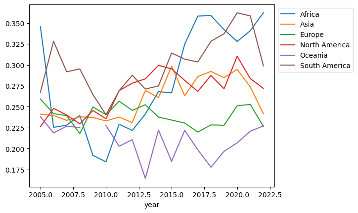
Here’s a plot to visualize the median negative emotional experiences by continent over the years. You’ll note that some of the lines are not contiguous — there are missing values. Let’s see if we can devise a plan to deal with this.
def get_continent(country_name):
    africa = ['Algeria', 'Angola', 'Benin', 'Botswana', 'Burkina Faso', 'Burundi', 'Cameroon', 'Central African Republic', 'Chad', 'Comoros', 'Congo (Brazzaville)', 'Congo (Kinshasa)', 'Djibouti', 'Egypt', 'Eswatini', 'Ethiopia', 'Gabon', 'Gambia', 'Ghana', 'Guinea', 'Ivory Coast', 'Kenya', 'Lesotho', 'Liberia', 'Libya', 'Madagascar', 'Malawi', 'Mali', 'Mauritania', 'Mauritius', 'Morocco', 'Mozambique', 'Namibia', 'Niger', 'Nigeria', 'Rwanda', 'Senegal', 'Seychelles', 'Sierra Leone', 'Somalia', 'Somaliland region', 'South Africa', 'South Sudan', 'Sudan', 'Tanzania', 'Togo', 'Tunisia', 'Uganda', 'Zambia', 'Zimbabwe']
    asia = ['Afghanistan', 'Armenia', 'Azerbaijan', 'Bahrain', 'Bangladesh', 'Bhutan', 'Cambodia', 'China', 'Cyprus', 'Georgia', 'Hong Kong S.A.R. of China', 'India', 'Indonesia', 'Iran', 'Iraq', 'Israel', 'Japan', 'Jordan', 'Kazakhstan', 'Kuwait', 'Kyrgyzstan', 'Laos', 'Lebanon', 'Malaysia', 'Maldives', 'Mongolia', 'Myanmar', 'Nepal', 'North Korea', 'Oman', 'Pakistan', 'Palestinian Territories', 'Philippines', 'Qatar', 'Saudi Arabia', 'Singapore', 'South Korea', 'Sri Lanka', 'State of Palestine', 'Syria', 'Taiwan Province of China', 'Tajikistan', 'Thailand', 'Turkiye', 'Turkmenistan', 'United Arab Emirates', 'Uzbekistan', 'Vietnam', 'Yemen']
    europe = ['Albania', 'Andorra', 'Austria', 'Belarus', 'Belgium', 'Bosnia and Herzegovina', 'Bulgaria', 'Croatia', 'Czechia', 'Denmark', 'Estonia', 'Finland', 'France', 'Germany', 'Greece', 'Hungary', 'Iceland', 'Ireland', 'Italy', 'Kosovo', 'Latvia', 'Liechtenstein', 'Lithuania', 'Luxembourg', 'Malta', 'Moldova', 'Monaco', 'Montenegro', 'Netherlands', 'North Macedonia', 'Norway', 'Poland', 'Portugal', 'Romania', 'Russia', 'San Marino', 'Serbia', 'Slovakia', 'Slovenia', 'Spain', 'Sweden', 'Switzerland', 'Ukraine', 'United Kingdom', 'Vatican City']
    n_america = ['Antigua and Barbuda', 'Bahamas', 'Barbados', 'Belize', 'Canada', 'Costa Rica', 'Cuba', 'Dominica', 'Dominican Republic', 'El Salvador', 'Grenada', 'Guatemala', 'Haiti', 'Honduras', 'Jamaica', 'Mexico', 'Nicaragua', 'Panama', 'Saint Kitts and Nevis', 'Saint Lucia', 'Saint Vincent and the Grenadines', 'Trinidad and Tobago', 'United States']
    s_america = ['Argentina', 'Bolivia', 'Brazil', 'Chile', 'Colombia', 'Ecuador', 'Guyana', 'Paraguay', 'Peru', 'Suriname', 'Uruguay', 'Venezuela']
    oceania = ['Australia', 'Fiji', 'Kiribati', 'Marshall Islands', 'Micronesia', 'Nauru', 'New Zealand', 'Palau', 'Papua New Guinea', 'Samoa', 'Solomon Islands', 'Tonga', 'Tuvalu', 'Vanuatu']

    if country_name in africa:
        return 'Africa'
    elif country_name in asia:
        return 'Asia'
    elif country_name in europe:
        return 'Europe'
    elif country_name in n_america:
        return 'North America'
    elif country_name in s_america:
        return 'South America'
    elif country_name in oceania:
        return 'Oceania'
    else:
        return 'Unknown'

(df
 .assign(Continent=df['Country name'].apply(get_continent))
 .groupby(['year', 'Continent'])
 ['Negative affect']
 .median()
 .unstack()
 .plot()
 .legend(bbox_to_anchor=(1,1))
)
Identifying Missing Values
Before proceeding, let’s identify if there are any missing values in the dataset. You can find out which columns contain missing values using the following pandas code:
# Identify missing values
df.isna().sum()
Country name 0
year 0
Life Ladder 0
Log GDP per capita 20
Social support 13
Healthy life expectancy at birth 54
Freedom to make life choices 33
Generosity 73
Perceptions of corruption 116
Positive affect 24
Negative affect 16
dtype: int64In Python, boolean valuesTrueandFalseare treated as 1 and 0, respectively, when used in numerical calculations. Therefore, when you use.sumon a DataFrame ofTrueandFalsevalues, it effectively counts the number ofTruevalues by summing them up as 1s, while theFalsevalues contribute zero to the sum.
This command returns a Series with the column names in the index and the number of missing values for column.
I also like to take the mean to quantify the percent missing:
# Identify missing values
df.isna().mean().mul(100)
Country name 0.000000
year 0.000000
Life Ladder 0.000000
Log GDP per capita 0.909504
Social support 0.591178
Healthy life expectancy at birth 2.455662
Freedom to make life choices 1.500682
Generosity 3.319691
Perceptions of corruption 5.275125
Positive affect 1.091405
Negative affect 0.727603
dtype: float64It looks with many columns are missing 1-5% of the time.
Armed with Python’s boolean mathematics, we can also count the missing values per row.
df.isna().sum(axis='columns')0 0
1 0
2 0
3 0
4 0
..
2194 0
2195 0
2196 0
2197 0
2198 0
Length: 2199, dtype: int64Let's throw a quick .value_counts on that to try and make sense of how many values might be missing for rows:
(df
 .isna()
 .sum(axis='columns')
 .value_counts()
)
0 1958
1 179
2 33
3 23
6 5
5 1
Name: count, dtype: int64It looks like most rows aren’t missing any values, but five rows are missing six values!
We could use a filter with .loc to examine which rows are missing three values:
(df
 .loc[df.isna().sum(axis='columns') == 3])
Country name year Life Ladder Log GDP per capita Social support Healthy life expectancy at birth Freedom to make life choices Generosity Perceptions of corruption Positive affect Negative affect
29 Algeria 2010 5.463567 9.306355 <NA> 65.5 0.592696 -0.209753 0.618038 <NA> <NA>
32 Algeria 2014 6.354898 9.355415 0.818189 65.900002 <NA> <NA> <NA> 0.558359 0.176866
33 Algeria 2016 5.340854 9.383312 0.748588 66.099998 <NA> <NA> <NA> 0.565026 0.377112
381 China 2006 4.560495 8.696139 0.747011 65.660004 <NA> <NA> <NA> 0.657659 0.16958
475 Cuba 2006 5.417869 <NA> 0.969595 68.0 0.281458 <NA> <NA> 0.596187 0.276602
524 Djibouti 2010 5.005811 7.934187 <NA> 54.599998 0.76373 -0.068953 0.59691 <NA> <NA>
992 Jordan 2018 4.638934 9.167903 0.799544 67.599998 0.76242 -0.1868 <NA> <NA> <NA>
993 Jordan 2019 4.452548 9.164418 0.79256 67.599998 0.725756 -0.165088 <NA> <NA> <NA>
994 Jordan 2020 4.093992 9.127326 0.70884 67.599998 0.778533 -0.151104 <NA> <NA> <NA>
1031 Kosovo 2007 5.103906 <NA> 0.847812 <NA> 0.381364 <NA> 0.894462 0.613723 0.236699
1207 Maldives 2018 5.197575 9.892906 0.913315 69.775002 0.854759 0.015678 <NA> <NA> <NA>
1323 Morocco 2010 4.383247 8.672808 <NA> 62.5 0.6629 -0.15965 0.900453 <NA> <NA>
1485 Oman 2011 6.852982 10.53862 <NA> 62.34 0.916293 0.009673 <NA> <NA> 0.295164
1755 Somaliland region 2009 4.991400 <NA> 0.879567 <NA> 0.746304 <NA> 0.513372 0.707874 0.112012
1756 Somaliland region 2010 4.657363 <NA> 0.829005 <NA> 0.820182 <NA> 0.471094 0.631947 0.083426
1757 Somaliland region 2011 4.930572 <NA> 0.787962 <NA> 0.858104 <NA> 0.357341 0.690514 0.122244
1758 Somaliland region 2012 5.057314 <NA> 0.786291 <NA> 0.758219 <NA> 0.333832 0.686732 0.152428
1842 State of Palestine 2022 4.907760 <NA> 0.859655 <NA> 0.694853 <NA> 0.835795 0.584111 0.361776
1897 Taiwan Province of China 2020 6.751068 <NA> 0.900833 <NA> 0.798835 <NA> 0.710567 0.743169 0.082737
1898 Taiwan Province of China 2021 6.246744 <NA> 0.866298 <NA> 0.818467 <NA> 0.675439 0.667417 0.12298
1899 Taiwan Province of China 2022 6.607147 <NA> 0.88282 <NA> 0.800192 <NA> 0.657556 0.716587 0.095399
1966 Tunisia 2009 5.025470 9.237887 <NA> 66.220001 0.781496 -0.124444 0.722211 <NA> <NA>
2044 United Arab Emirates 2013 6.620951 11.040596 0.863716 65.279999 0.935979 <NA> <NA> <NA> 0.291113When to Drop Data
Ah, the million-dollar question: When should you use the pandas dropna method?
There are textbooks devoted to this subject. To keep this post short and focus on removing data with .dropna, I will summarize when we can drop rows: when the missingness of data has no relation with any observed or unobserved variables. In simpler terms, the data is missing purely by chance. It's the most straightforward form of missing data to manage because you can generally remove it without biasing your results if it is a small percentage of the data.
When should we drop columns? Again, in short, when they don’t add value. However, I would not use pandas dropna to remove columns even if I could. I would do exploratory data analysis (EDA), determine which columns I care about, and then use pandas loc to select those columns. (See my previous posts on pandas loc and pandas iloc for details.)
Here is a function for determining whether data is missing completely at random (MCAR).
import pandas as pd
from scipy.stats import ttest_ind
import warnings

def is_mcar(df, column, p_value_threshold=0.05):
    """
    Assess whether a column in a DataFrame is Missing Completely At Random (MCAR) using t-tests.

    Parameters:
    df (pandas.DataFrame): The DataFrame containing the data.
    column (str): The column name to assess for MCAR.
    p_value_threshold (float): The p-value above which to consider data as potentially MCAR. Default is 0.05.

    Returns:
    bool: True if the column is likely MCAR, False otherwise.
    """

    # Check if the column has missing values
    if df[column].isna().sum() == 0:
        warnings.warn(f"The column '{column}' has no missing values.")
        return False

    def ttest_helper(sub_df, column):
        mcar = True
        for col in sub_df.select_dtypes(include=['number']).columns:
            if col == column or col == 'Is_Missing':
                continue
            group1 = (sub_df
                      .loc[sub_df['Is_Missing'] == True, col]
                      .dropna()
                     )
            group2 = (sub_df
                      .loc[sub_df['Is_Missing'] == False, col]
                      .dropna()
                     )
            if len(group1) > 1 and len(group2) > 1:
                t_stat, p_value = ttest_ind(group1, group2)
                if p_value < p_value_threshold:
                    mcar = False
                    break
        return mcar

    return (df.assign(Is_Missing=df[column].isna())
              .pipe(ttest_helper, column)
           )
The function is_mcar takes a column and use a special test called a "t-test" to compare the people with missing scores to those with available scores, but using other numerical information we have from the columns, like health, income, or family support. If the test finds no real difference between the two groups, the missing column scores are probably just random and not tied to any of the other factors we're looking at. In that case, we say this data is "Missing Completely At Random" (MCAR).
Let’s run it on all of the columns:
for col in df.columns:
    print(f'{col=} {is_mcar(df, col)}')
col='Country name' False
col='year' False
col='Life Ladder' False
col='Log GDP per capita' False
col='Social support' False
col='Healthy life expectancy at birth' False
col='Freedom to make life choices' False
col='Generosity' False
col='Perceptions of corruption' False
col='Positive affect' False
col='Negative affect' True
/var/folders/qn/r8_0pgj1645dn1w69vqls6cw0000gn/T/ipykernel_54500/3428414951.py:20: UserWarning: The column 'Country name' has no missing values.
warnings.warn(f"The column '{column}' has no missing values.")
/var/folders/qn/r8_0pgj1645dn1w69vqls6cw0000gn/T/ipykernel_54500/3428414951.py:20: UserWarning: The column 'year' has no missing values.
warnings.warn(f"The column '{column}' has no missing values.")
/var/folders/qn/r8_0pgj1645dn1w69vqls6cw0000gn/T/ipykernel_54500/3428414951.py:20: UserWarning: The column 'Life Ladder' has no missing values.
warnings.warn(f"The column '{column}' has no missing values.")Because .72% of the Negative affect values are missing completely at random, I’m going to remove those rows.
(df
 .dropna(subset='Negative affect')
)
Country name year Life Ladder Log GDP per capita Social support Healthy life expectancy at birth Freedom to make life choices Generosity Perceptions of corruption Positive affect Negative affect
0 Afghanistan 2008 3.723590 7.350416 0.450662 50.500000 0.718114 0.167652 0.881686 0.414297 0.258195
1 Afghanistan 2009 4.401778 7.508646 0.552308 50.799999 0.678896 0.190809 0.850035 0.481421 0.237092
2 Afghanistan 2010 4.758381 7.613900 0.539075 51.099998 0.600127 0.121316 0.706766 0.516907 0.275324
3 Afghanistan 2011 3.831719 7.581259 0.521104 51.400002 0.495901 0.163571 0.731109 0.479835 0.267175
4 Afghanistan 2012 3.782938 7.660506 0.520637 51.700001 0.530935 0.237588 0.775620 0.613513 0.267919
... ... ... ... ... ... ... ... ... ... ... ...
2194 Zimbabwe 2018 3.616480 7.783066 0.775388 52.625000 0.762675 -0.051219 0.844209 0.657524 0.211726
2195 Zimbabwe 2019 2.693523 7.697755 0.759162 53.099998 0.631908 -0.047464 0.830652 0.658434 0.235354
2196 Zimbabwe 2020 3.159802 7.596050 0.717243 53.575001 0.643303 0.006313 0.788523 0.660658 0.345736
2197 Zimbabwe 2021 3.154578 7.656878 0.685151 54.049999 0.667636 -0.075575 0.756945 0.609917 0.241682
2198 Zimbabwe 2022 3.296220 7.670123 0.666172 54.525002 0.651987 -0.069513 0.752632 0.640609 0.191350
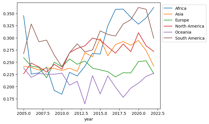
2183 rows × 11 columnsLet’s redo the plot with the cleaned up data:
(df
 .dropna(subset='Negative affect')
 .assign(Continent=df['Country name'].apply(get_continent))
 .groupby(['year', 'Continent'])
 ['Negative affect']
 .median()
 .unstack()
 .plot()
 .legend(bbox_to_anchor=(1,1))
)
There is still a gap in the Oceania line. Let’s explore that and see the rows with missing values:
(df
 .dropna(subset='Negative affect')
 .assign(Continent=df['Country name'].apply(get_continent))
 .groupby(['year', 'Continent'])
 ['Negative affect']
 .median()
 .unstack()
)
Continent Africa Asia Europe North America Oceania South America
year
2005 0.345555 0.241056 0.259164 0.226111 0.238012 0.267397
2006 0.225375 0.239390 0.241685 0.248030 0.218773 0.328230
2007 0.227878 0.233697 0.239325 0.240080 0.226674 0.291755
2008 0.239573 0.237846 0.217813 0.229474 0.225154 0.295163
2009 0.191887 0.237092 0.249777 0.245432 <NA> 0.264550
2010 0.184129 0.233014 0.240364 0.235618 0.227416 0.240530
2011 0.229093 0.237561 0.256577 0.269225 0.202737 0.269106
2012 0.221627 0.231071 0.245632 0.278111 0.210638 0.287592
2013 0.241231 0.269507 0.252374 0.283281 0.16427 0.271086
2014 0.268049 0.260893 0.237620 0.299388 0.222162 0.274822
2015 0.266510 0.298386 0.234048 0.295253 0.184733 0.314151
2016 0.324739 0.263090 0.230485 0.281422 0.22175 0.306865
2017 0.358310 0.286023 0.219717 0.268269 0.198539 0.303513
2018 0.358828 0.292183 0.228276 0.287358 0.177704 0.328171
2019 0.342163 0.284670 0.227838 0.271475 0.196683 0.337148
2020 0.327903 0.294512 0.251109 0.310301 0.206809 0.362144
2021 0.340848 0.273718 0.252777 0.283584 0.220745 0.358491
2022 0.362231 0.241539 0.226395 0.271906 0.227067 0.298878It looks like data is missing from 2009. Let’s look at the non-aggregated values from Oceania from 2009:
(df
 .dropna(subset='Negative affect')
 .assign(Continent=df['Country name'].apply(get_continent))
 .query('Continent == "Oceania" and 2008 <= year <= 2010')
)
Country name year Life Ladder Log GDP per capita Social support Healthy life expectancy at birth Freedom to make life choices Generosity Perceptions of corruption Positive affect Negative affect Continent
78 Australia 2008 7.253757 10.709456 0.946635 70.040001 0.915733 0.301722 0.430811 0.728992 0.218427 Oceania
79 Australia 2010 7.450047 10.713649 0.954520 70.199997 0.932059 0.313121 0.366127 0.761716 0.220073 Oceania
1398 New Zealand 2008 7.381171 10.541654 0.944275 69.760002 0.893072 0.292630 0.333751 0.784192 0.231881 Oceania
1399 New Zealand 2010 7.223756 10.534310 0.975642 69.800003 0.917753 0.249289 0.320748 0.782821 0.234758 OceaniaThe rows for 2009 are completely missing for Australia and New Zealand. I’m not a subject matter expert on happiness, but since this is my blog post, I will make an executive decision and use the value from 2008 for 2009. The values surrounding it look close enough. We call this a forward fill because we will push the last known value forward. (A quick aside: if you are doing machine learning with time series, this is a popular choice for dealing with missing values because it doesn’t leak information from the future.)
Here’s the plot with the values filled in:
(df
 .dropna(subset='Negative affect')
 .assign(Continent=df['Country name'].apply(get_continent))
 .groupby(['year', 'Continent'])
 ['Negative affect']
 .median()
 .unstack()
 .assign(Oceania=lambda df_:df_.Oceania.ffill())
 .plot()
 .legend(bbox_to_anchor=(1,1))
)
This plot is ok. However, I want to fix the labels, and draw focus to the Europe values:
import matplotlib.pyplot as plt
from matplotlib.ticker import MaxNLocator

column_colors = []

def get_column_names_and_set_colors(df):
    global column_colors
    for col in df.columns:
        if col == 'Europe':
            column_colors.append('red')
        else:
            column_colors.append('grey')

    return df

ax = (df
      .dropna(subset=['Negative affect'])
      .assign(Continent=df['Country name'].apply(get_continent))
      .groupby(['year', 'Continent'])
      ['Negative affect']
      .median()
      .unstack()
      .pipe(get_column_names_and_set_colors)
      .assign(Oceania=lambda df_:df_.Oceania.ffill())
      .plot(linewidth=2, color=column_colors)
)

# Set x-axis to display whole numbers only
ax.xaxis.set_major_locator(MaxNLocator(integer=True))

# Move the legend box outside of the plot area
ax.legend(bbox_to_anchor=(1, 1))
ax.set_title('Median Negative affect in European Countries')
ax.set_ylabel('negative affect')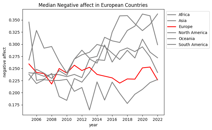
That looks better. The negative affect in Europe has held pretty constant while other continents have seen it rising since 2010.
Dropping Entirely Empty Rows
Let me show you another place .dropna comes in useful.
Imagine you’ve just downloaded an exciting new dataset that you can’t wait to dive into. You load it into a DataFrame, only to find several empty rows at the end. All fields are missing or set to a ‘null’ value in these rows. I find this occasionally happens to me.
Here is a toy example:
import pandas as pd
from io import StringIO

csv_string = """Name,Age,Income
Alice,34,50000
Bob,45,75000
Cathy,,120000
Dave,31,60000
,,
,,
,,"""


df_empty = pd.read_csv(StringIO(csv_string))
df_empty
Name Age Income
0 Alice 34.0 50000.0
1 Bob 45.0 75000.0
2 Cathy NaN 120000.0
3 Dave 31.0 60000.0
4 NaN NaN NaN
5 NaN NaN NaN
6 NaN NaN NaNIf my data had a bunch of missing rows, I would use.dropnabut with a specific incantation, specifyinghow='all'. This only removes rows if every cell is missing. Note that Cathy was missing Age but not dropped:
df_empty.dropna(how='all') Name Age Income
0 Alice 34.0 50000.0
1 Bob 45.0 75000.0
2 Cathy NaN 120000.0
3 Dave 31.0 60000.0Conclusion
Handling missing data is a crucial part of the data preprocessing pipeline, and the pandas dropna method offers a flexible way to manage such data. Understanding the nature of your missing values is essential for making informed decisions. The pandas dropna method is a blunt tool; you must be careful before dropping values. Remember, each dataset has challenges, and there’s no one-size-fits-all solution. Best of luck in keeping around data that sparks joy!
If you liked this, check out our previous Professional Pandas posts on Pandas iloc, Pandas loc, the Pandas merge method, and the Pandas assign method / chaining.