

Introduction to Pandas Iloc
In this post, I describe how Pandas iloc (.iloc) can be used for indexing, but I also argue that you rarely need to use it. There are almost always cleaner options.
We start by giving a high-level description of Pandas iloc. Then we discuss each of the possible input types, with examples. And finally, we talk about the dangers of magic numbers (numbers that appear in your code with no explanation). Throughout, I’ll present alternatives to Pandas iloc and describe why I think they’re more useful.
This is the fourth piece in our Professional Pandas series on teaching best practices about writing professional-grade Pandas code, and a follow-up to a companion piece on Pandas Loc. If you have questions or topics that you would like to dive into, please reach out on Twitter to @ponderdata or @__mharrison__, and if you’d like to see the notebook version of this blogpost, you can find it on Github here.
Try Ponder Today
Start running your Python data science workflows in your database within minutes!
Table of Contents
- Introduction to Pandas Iloc
- What Is Pandas Iloc?
- What Inputs Does Pandas Iloc Accept?
- How to Use Pandas Iloc with Each Input Type
- Part 1: Using Pandas Iloc to Index with an Integer (e.g., 5)
- Part 2: Using Pandas Iloc to Index with a List or Array of Integers (e.g., [4, 3, 0])
- Part 3: Using Pandas Iloc to Index with a Slice Object with Ints (e.g., 1:7)
- Part 4: Using Pandas Iloc to Index with a Boolean Array
- Part 5: Using Pandas Iloc to Index with a Callable Function
- Part 6: Using Pandas Iloc to Index with a Tuple
- Code Readability and the Danger of Magic Numbers
- Conclusion
What is Pandas Iloc?
.iloc stands for integer location. Often folks say it is used to subset a portion of a dataframe or series. We can use it to pull out rows or columns based on location.You will hear this referred to as a function or a method. Both of those are incorrect. Pandas iloc is a property, and we leverage the property by using an index operation (this is with square brackets). You are probably familiar with indexing dictionaries, lists, or strings.
For example, to find the first character of a string, we can do this:
>>> name = 'Matt'
>>> name[0]
'M'
Or we can get the last item in a list with an index of -1:
>>> names = ['Paul', 'George', 'Ringo', 'John']
>>> name[-1]
'John'
Indexing with.ilocdiffers from indexing with a string or list. A list is one-dimensional while a dataframe is two-dimensional and you can slice it in both dimensions at once..iloctakes up to two arguments: the row index selector (required) and an optional column index selector (by passing in a tuple). Pandas recognizes if you pass in a tuple and slices in two dimensions. You can't do this with lists or strings.
Inside the brackets following .iloc, you can place a row selector and an optional column selector. The syntax looks like this:
dataframe.iloc[row_selector, column_selector]While.ilocleverages integer-based indexing, Pandas offers other indexing functions. You can index directly on DataFrames, Series, and GroupBy objects. But you can also use.loc.
We discussed label-based indexing with Pandas loc in our last professional Pandas post. Pandas loc uses labels instead of integer positions to select data.
A Strong Opinion: Don’t Use Pandas Iloc in Production
I find myself using.ilocfor inspection and exploratory data analysis and not for production operations. Generally, I suggest you leverage.locinstead of.ilocbecause it is more explicit and less error-prone.
As we go through the many.ilocexamples in the post, I'll show alternatives that I think are cleaner, but here's one sneak peak: Some people use.ilocto pull off the top 10 or bottom 10 entries, but I prefer to use.heador.tailbecause they are more explicit.
What Inputs Does Pandas Iloc Accept?
Given that caveat, let's explore options for .iloc. I will try to include real-world examples gleaned from my hard drive.
The documentation states that we can index with the following values (and what follows are direct quotes):
- An integer, e.g.
5. - A list or array of integers, e.g.
[4, 3, 0]. - A slice object with ints, e.g.
1:7. - A boolean array.
- A
callablefunction with one argument (the calling Series or DataFrame) and that returns valid output for indexing (one of the above). This is useful in method chains, when you don’t have a reference to the calling object, but would like to base your selection on some value. - A tuple of row and column indexes. The tuple elements consist of one of the above inputs, e.g.
(0, 1).
Let’s see how these work.
How to Use Pandas Iloc with Each Input Type
Part 1: Using Pandas Iloc to Index with an Integer (e.g., 5)
Here is an example that pulls out rows of a stock using an integer. Let’s load Pandas and the data. This data is daily stock data from the first half of 2023.
import pandas as pd

url = 'https://github.com/mattharrison/datasets/raw/master/data/tickers-raw.csv'
price_df = pd.read_csv(url)

price_df
Date BRK-B DIS F IBM MMM NFLX PG QCOM TSLA UPS ^GSPC
0 2022-12-22 00:00:00-05:00 302.69 86.67 10.51 137.30 118.20 297.75 150.30 109.25 125.35 172.42 3822.39
1 2022-12-23 00:00:00-05:00 306.49 88.01 10.55 138.05 116.79 294.96 150.72 109.41 123.15 173.79 3844.82
2 2022-12-27 00:00:00-05:00 305.55 86.37 10.41 138.80 116.87 284.17 152.04 108.05 109.10 173.72 3829.25
3 2022-12-28 00:00:00-05:00 303.43 84.17 10.17 136.46 115.00 276.88 150.07 105.59 112.71 170.46 3783.22
4 2022-12-29 00:00:00-05:00 309.06 87.18 10.72 137.47 117.21 291.12 150.69 108.42 121.82 172.56 3849.28
... ... ... ... ... ... ... ... ... ... ... ... ...
119 2023-06-15 00:00:00-04:00 339.82 92.94 14.45 138.40 103.81 445.27 148.45 123.61 255.90 179.00 4425.84
120 2023-06-16 00:00:00-04:00 338.31 91.32 14.42 137.48 104.54 431.96 149.54 122.68 260.54 178.58 4409.59
121 2023-06-20 00:00:00-04:00 338.67 89.75 14.22 135.96 102.30 434.70 148.16 119.82 274.45 177.27 4388.71
122 2023-06-21 00:00:00-04:00 338.61 88.64 14.02 133.69 101.47 424.45 149.44 115.76 259.46 173.63 4365.69
123 2023-06-22 00:00:00-04:00 336.91 88.39 14.28 130.91 100.27 420.61 149.79 116.36 261.47 172.37 4368.72
124 rows × 12 columnsHere is the code example, from the book Algorithmic Short Selling with Python.
The first row stores the Cost of the stock in another dataframe. The last row gets the current Price of a stock. (Don't try to run this one -- We haven't initialized a dataframe called port, so you'll get an error.)
port['Cost'] = price_df.iloc[0,:]
port['Price'] = price_df.iloc[-1,:]
You can see that the0and-1are the row selectors. This first example should pull out the first row. Because Pandas doesn't really have a datatype for a row, it presents it as a series.
price_df.iloc[0,:]Date 2022-12-22 00:00:00-05:00
BRK-B 302.69
DIS 86.67
F 10.51
IBM 137.3
MMM 118.2
NFLX 297.75
PG 150.3
QCOM 109.25
TSLA 125.35
UPS 172.42
^GSPC 3822.39
Name: 0, dtype: objectThe author of this code included a slice for the column selector as well. The bare slice, :, selects all of the columns. (Which is unneeded in this code). This returns a single row of a dataframe. This code does the same without requiring the column selector:
price_df.iloc[0]Date 2022-12-22 00:00:00-05:00
BRK-B 302.69
DIS 86.67
F 10.51
IBM 137.3
MMM 118.2
NFLX 297.75
PG 150.3
QCOM 109.25
TSLA 125.35
UPS 172.42
^GSPC 3822.39
Name: 0, dtype: objectNote that if you pass in a list with 0 in it for the row selector, you get back a dataframe with a single row, which is the type we will explore in the next section:
price_df.iloc[[0]] Date BRK-B DIS F IBM MMM NFLX PG QCOM TSLA UPS ^GSPC
0 2022-12-22 00:00:00-05:00 302.69 86.67 10.51 137.3 118.2 297.75 150.3 109.25 125.35 172.42 3822.39Part 2: Using Pandas Iloc to Index with a List or Array of Integers (e.g., [4, 3, 0])
If you pass in a list of integers to the row selector, Pandas will return a dataframe with rows from those positions. You can also pass in a list of integer positions for column selectors.
I looked through my hard drive and had a hard time coming up with an example for this. So I searched further, and found one in the Pandas source code.
This is the test_sort_values_categorical method that tests if sorting works (pandas/tests/series/methods/test_sort_values.py). It uses Pandas iloc to manually re-arrange the rows by hardcoded values so they are in the correct order:
# multi-columns sort
# GH#7848
df = DataFrame(
    {"id": [6, 5, 4, 3, 2, 1], "raw_grade": ["a", "b", "b", "a", "a", "e"]}
)
df["grade"] = Categorical(df["raw_grade"], ordered=True)
df["grade"] = df["grade"].cat.set_categories(["b", "e", "a"])

# sorts 'grade' according to the order of the categories
result = df.sort_values(by=["grade"])
expected = df.iloc[[1, 2, 5, 0, 3, 4]]
tm.assert_frame_equal(result, expected)
This is actually a good use for.iloc. It is small, synthetic, and easy to understand. In the real world, I have much bigger data and manually reordering the rows by index wouldn't make sense. Hence the.sort_valuesmethod.
Note that you can repeat rows or columns using .iloc:
vehicle_url = 'https://github.com/mattharrison/datasets/raw/master/data/vehicles.csv.zip'
df = pd.read_csv(vehicle_url)
df barrels08 barrelsA08 charge120 charge240 city08 city08U cityA08 cityA08U cityCD cityE ... mfrCode c240Dscr charge240b c240bDscr createdOn modifiedOn startStop phevCity phevHwy phevComb
0 15.695714 0.0 0.0 0.0 19 0.0 0 0.0 0.0 0.0 ... NaN NaN 0.0 NaN Tue Jan 01 00:00:00 EST 2013 Tue Jan 01 00:00:00 EST 2013 NaN 0 0 0
1 29.964545 0.0 0.0 0.0 9 0.0 0 0.0 0.0 0.0 ... NaN NaN 0.0 NaN Tue Jan 01 00:00:00 EST 2013 Tue Jan 01 00:00:00 EST 2013 NaN 0 0 0
2 12.207778 0.0 0.0 0.0 23 0.0 0 0.0 0.0 0.0 ... NaN NaN 0.0 NaN Tue Jan 01 00:00:00 EST 2013 Tue Jan 01 00:00:00 EST 2013 NaN 0 0 0
3 29.964545 0.0 0.0 0.0 10 0.0 0 0.0 0.0 0.0 ... NaN NaN 0.0 NaN Tue Jan 01 00:00:00 EST 2013 Tue Jan 01 00:00:00 EST 2013 NaN 0 0 0
4 17.347895 0.0 0.0 0.0 17 0.0 0 0.0 0.0 0.0 ... NaN NaN 0.0 NaN Tue Jan 01 00:00:00 EST 2013 Tue Jan 01 00:00:00 EST 2013 NaN 0 0 0
... ... ... ... ... ... ... ... ... ... ... ... ... ... ... ... ... ... ... ... ... ...
41139 14.982273 0.0 0.0 0.0 19 0.0 0 0.0 0.0 0.0 ... NaN NaN 0.0 NaN Tue Jan 01 00:00:00 EST 2013 Tue Jan 01 00:00:00 EST 2013 NaN 0 0 0
41140 14.330870 0.0 0.0 0.0 20 0.0 0 0.0 0.0 0.0 ... NaN NaN 0.0 NaN Tue Jan 01 00:00:00 EST 2013 Tue Jan 01 00:00:00 EST 2013 NaN 0 0 0
41141 15.695714 0.0 0.0 0.0 18 0.0 0 0.0 0.0 0.0 ... NaN NaN 0.0 NaN Tue Jan 01 00:00:00 EST 2013 Tue Jan 01 00:00:00 EST 2013 NaN 0 0 0
41142 15.695714 0.0 0.0 0.0 18 0.0 0 0.0 0.0 0.0 ... NaN NaN 0.0 NaN Tue Jan 01 00:00:00 EST 2013 Tue Jan 01 00:00:00 EST 2013 NaN 0 0 0
41143 18.311667 0.0 0.0 0.0 16 0.0 0 0.0 0.0 0.0 ... NaN NaN 0.0 NaN Tue Jan 01 00:00:00 EST 2013 Tue Jan 01 00:00:00 EST 2013 NaN 0 0 0
41144 rows × 83 columnsdf.iloc[[0,0,1,0], [-1, 1, 1]] phevComb barrelsA08 barrelsA08
0 0 0.0 0.0
0 0 0.0 0.0
1 0 0.0 0.0
0 0 0.0 0.0Part 3: Using Pandas Iloc to Index with a Slice Object with Ints (e.g., 1:7)
Generally, when code uses slices with.iloc, it is pulling off the first or last rows..iloc[:5]will return the first five rows. (Rows from positions 0, 1, 2, 3, and 4.) Note that this is the half-open interval. It includes the first position (0 if not defined) and up to but not including the last position.
This also works for the column selector. .iloc[7:20, -5:] returns 13 rows starting at index position 7 (the eighth row) and the last five columns. One of the nice attributes of the half-open interval is that the length of the result is the end of the slice minus the first part of the slice. 20 minus seven is 13.
A negative index position means count back from the end. You could usedf.iloc[:, 81:83]if you want the last two columns of a dataframe with 83 columns, or you could usedf.iloc[:, -2:]. The-2could be interpreted aslen(columns)-2or 81. The bare slice for the row selector, :, returns all of the rows.
But again, there are better options than Pandas iloc: 95% of.ilocusage with slices of rows can be replaced with.heador.tailand improve readability substantially.
Here’s a longer example of code I use when doing principal component analysis (PCA) visualization. Let’s run PCA on the Fuel Economy data from the US government. (We’ll see Pandas iloc come into play when it comes time to visualize the PCA results.)
from feature_engine import encoding
from sklearn import base, compose, pipeline, preprocessing, set_config
from sklearn.decomposition import PCA
from sklearn.preprocessing import StandardScaler
set_config(transform_output='pandas')
def tweak_autos(autos):
cols = ['city08', 'comb08', 'highway08', 'cylinders', 'displ', 'drive', 'eng_dscr',
'fuelCost08', 'make', 'model', 'trany', 'range', 'createdOn', 'year']
return (autos
[cols]
.assign(cylinders=autos.cylinders.fillna(0).astype('int8'),
displ=autos.displ.fillna(0).astype('float16'),
drive=autos.drive.fillna('Other').astype('category'),
automatic=autos.trany.str.contains('Auto').fillna(0).astype('int8'),
speeds=autos.trany.str.extract(r'(\d)+').fillna('20').astype('int8'),
createdOn=pd.to_datetime(autos.createdOn.replace({' EDT': '-04:00',
' EST': '-05:00'}, regex=True), utc=True).dt.tz_convert('America/New_York'),
ffs=autos.eng_dscr.str.contains('FFS').fillna(0).astype('int8')
)
.astype({'highway08': 'int8', 'city08': 'int16', 'comb08': 'int16', 'fuelCost08':
'int16',
'range': 'int16', 'year': 'int16', 'make': 'category'})
.loc[:, ['city08', 'comb08', 'highway08', 'cylinders', 'displ', 'drive',
'fuelCost08', 'make', 'model', 'range', 'createdOn', 'year',
'automatic', 'speeds', 'ffs']]
)
class TweakTransformer(base.BaseEstimator, base.TransformerMixin):
def fit(self, X):
return self
def transform(self, X):
return tweak_autos(X)
def get_pipeline():
categorical_features = ['drive', 'make', 'model']
numeric_features = ['city08', 'comb08', 'highway08',
'cylinders', 'displ', 'fuelCost08',
'range', 'year', 'automatic', 'speeds', 'ffs']
num_pipeline = pipeline.Pipeline(steps=[
('std', preprocessing.StandardScaler())
])
cat_pipeline = pipeline.Pipeline(steps=[
('oh', encoding.OneHotEncoder(top_categories=5, drop_last=True))
])
pipe = pipeline.Pipeline([
('tweak', TweakTransformer()),
('ct', compose.ColumnTransformer(transformers=[
('num', num_pipeline, numeric_features),
('cat', cat_pipeline, categorical_features),
])),
]
)
return pipe
def get_pca_pipeline():
scaler = StandardScaler()
pca = PCA()
pl = pipeline.make_pipeline(scaler, pca)
return plWith that code in place, let's make our cleanup pipeline to generate the data for machine learning, X:
pl = get_pipeline()
X = pl.fit_transform(df)
X
num__city08 num__comb08 num__highway08 num__cylinders num__displ num__fuelCost08 num__range num__year num__automatic num__speeds ... cat__make_Chevrolet cat__make_Ford cat__make_Dodge cat__make_GMC cat__make_Toyota cat__model_F150 Pickup 2WD cat__model_F150 Pickup 4WD cat__model_Mustang cat__model_Jetta cat__model_Truck 2WD
0 0.079809 0.049985 0.064077 -0.939606 -0.930490 -0.553207 -0.060845 -1.484011 -1.486392 -0.113886 ... 0 0 0 0 0 0 0 0 0 0
1 -1.185086 -1.253042 -1.358900 3.512290 1.180007 2.271333 -0.060845 -1.484011 -1.486392 -0.113886 ... 0 0 0 0 0 0 0 0 0 0
2 0.585768 0.831800 1.098970 -0.939606 -0.785428 -1.240257 -0.060845 -1.484011 -1.486392 -0.113886 ... 0 0 1 0 0 0 0 0 0 0
3 -1.058597 -1.253042 -1.617623 1.286342 1.399021 2.271333 -0.060845 -1.484011 0.672770 -0.909896 ... 0 0 1 0 0 0 0 0 0 0
4 -0.173170 -0.210621 -0.194646 -0.939606 -0.785428 0.515538 -0.060845 -0.766025 -1.486392 -0.113886 ... 0 0 0 0 0 0 0 0 0 0
... ... ... ... ... ... ... ... ... ... ... ... ... ... ... ... ... ... ... ... ... ...
41139 0.079809 0.180287 0.193439 -0.939606 -0.785428 -0.705884 -0.060845 -0.766025 0.672770 -0.511891 ... 0 0 0 0 0 0 0 0 0 0
41140 0.206299 0.310590 0.452162 -0.939606 -0.785428 -0.782223 -0.060845 -0.766025 -1.486392 -0.113886 ... 0 0 0 0 0 0 0 0 0 0
41141 -0.046680 0.049985 -0.065284 -0.939606 -0.785428 -0.553207 -0.060845 -0.766025 0.672770 -0.511891 ... 0 0 0 0 0 0 0 0 0 0
41142 -0.046680 0.049985 -0.065284 -0.939606 -0.785428 -0.553207 -0.060845 -0.766025 -1.486392 -0.113886 ... 0 0 0 0 0 0 0 0 0 0
41143 -0.299660 -0.340923 -0.453369 -0.939606 -0.785428 0.820894 -0.060845 -0.766025 0.672770 -0.511891 ... 0 0 0 0 0 0 0 0 0 0
41144 rows × 26 columnsOnce we have that data, let’s send it through our PCA pipeline, which standardizes the data and then feeds it to the PCA algorithm:
pca_pl = get_pca_pipeline()
pca_pl.fit_transform(X)
pca0 pca1 pca2 pca3 pca4 pca5 pca6 pca7 pca8 pca9 ... pca16 pca17 pca18 pca19 pca20 pca21 pca22 pca23 pca24 pca25
0 0.477062 -2.095174 0.770188 -0.212903 -0.951630 0.676938 -0.238926 0.289078 -0.740275 0.155848 ... 0.349791 -0.496253 0.237550 0.038151 0.212713 -0.236530 -0.012753 -0.174440 -0.007384 0.032632
1 -4.268353 0.083709 0.988989 -0.406348 -0.790531 0.107578 -0.072892 0.070620 -0.463815 0.187307 ... -0.679322 2.164472 0.463913 -0.271684 1.396367 0.003845 1.387906 -0.348073 -0.282840 -0.020434
2 2.223967 -2.811101 -0.325520 -0.617319 -0.598618 -1.267804 2.235811 0.444152 0.445463 1.456438 ... 0.114138 -0.023109 -0.611794 -0.436919 0.084360 -0.158280 0.081188 -0.178606 0.345765 -0.033851
3 -4.042764 -0.429124 1.000171 -1.017005 -0.974965 -1.251741 2.801752 -0.073256 0.909080 1.261115 ... -0.430511 -0.581322 -0.308522 0.426849 1.287281 0.616496 0.055086 -0.331410 -0.077058 -0.038770
4 -0.139146 -2.032831 -0.538644 -0.316546 1.840327 0.798375 -0.194294 0.064586 -0.862334 0.194610 ... 0.510479 -0.051578 0.403818 0.149321 -0.555183 0.342289 -0.105411 0.038149 0.184141 0.019709
... ... ... ... ... ... ... ... ... ... ... ... ... ... ... ... ... ... ... ... ... ...
41139 1.377499 -1.709720 -0.699271 0.007333 -0.305877 -0.638405 0.296353 0.026869 0.397360 -0.318153 ... 0.376670 0.103955 0.519335 0.167599 -0.254011 -0.122864 -0.182352 -0.038450 -0.003055 -0.039244
41140 1.748701 -2.100211 -0.734197 0.048718 -0.347412 -0.195885 -0.149926 0.314707 -0.301994 0.008568 ... -0.135854 0.938395 0.307274 0.093213 -0.328319 -0.172653 -0.215587 -0.025868 0.035057 -0.001246
41141 0.307412 -1.652104 -0.416253 -0.326038 1.831733 0.360856 0.128497 -0.178601 -0.178784 -0.122508 ... 1.101649 -1.133470 0.475791 -0.331684 -0.444559 -0.334098 -0.069290 -0.028727 0.083650 -0.072446
41142 0.450261 -2.073459 -0.552671 -0.268423 1.773376 0.814024 -0.303813 0.101635 -0.884443 0.196430 ... 0.564450 -0.309094 0.270824 -0.248844 -0.524381 -0.398215 -0.113874 -0.010273 0.008102 -0.069861
41143 -0.593758 -1.626213 -0.475329 -0.373315 1.902766 0.350590 0.274209 -0.229919 -0.155403 -0.130760 ... 1.017916 -0.824843 0.644316 0.279251 -0.484714 0.571243 -0.071891 0.035067 0.187376 -0.022398
41144 rows × 26 columnsHaving run PCA on the data, let’s look at the components that make up the weights to calculate the embeddings. (We’ll only display the first two as an example.)
pca_pl.named_steps['pca'].components_[0:2]array([[ 0.37501081, 0.38968423, 0.39554789, -0.34148913, -0.3483539 ,
-0.36421128, 0.19347438, 0.0875742 , -0.05200177, 0.07680492,
-0.03992407, 0.24258046, -0.17168667, -0.11188447, 0.04104331,
-0.01628179, -0.05080095, -0.03737196, -0.05577404, -0.09616649,
0.04123887, -0.03649398, -0.03769309, -0.01286445, 0.03708651,
0.00463668],
[ 0.05963524, 0.0652074 , 0.07807361, 0.19236311, 0.17215519,
0.07042231, 0.08233002, 0.54374148, 0.25799294, 0.3409357 ,
-0.49177226, -0.16771429, 0.05033319, -0.09918001, 0.292591 ,
0.20112942, -0.02188441, -0.05225876, -0.09589855, 0.01754167,
-0.03934466, -0.02033149, -0.03234882, -0.00660427, -0.01698125,
-0.0693592 ]])Let’s throw that into a dataframe to make it easier to understand. The rows represent the weights for columns for each principal component. The larger weights have more of an impact on the principal components.
def components_to_df(pca_components, feature_names):
    idxs = [f'PC{i}' for i in range(len(pca_components))]
    return pd.DataFrame(pca_components, columns=feature_names,
                            index=idxs)
comps = components_to_df(pca_pl.named_steps['pca'].components_, X.columns)
comps.head()
num__city08 num__comb08 num__highway08 num__cylinders num__displ num__fuelCost08 num__range num__year num__automatic num__speeds ... cat__make_Chevrolet cat__make_Ford cat__make_Dodge cat__make_GMC cat__make_Toyota cat__model_F150 Pickup 2WD cat__model_F150 Pickup 4WD cat__model_Mustang cat__model_Jetta cat__model_Truck 2WD
PC0 0.375011 0.389684 0.395548 -0.341489 -0.348354 -0.364211 0.193474 0.087574 -0.052002 0.076805 ... -0.050801 -0.037372 -0.055774 -0.096166 0.041239 -0.036494 -0.037693 -0.012864 0.037087 0.004637
PC1 0.059635 0.065207 0.078074 0.192363 0.172155 0.070422 0.082330 0.543741 0.257993 0.340936 ... -0.021884 -0.052259 -0.095899 0.017542 -0.039345 -0.020331 -0.032349 -0.006604 -0.016981 -0.069359
PC2 0.269448 0.235022 0.178760 0.130405 0.186508 0.123961 0.520875 -0.112167 0.020663 -0.230661 ... 0.079818 0.162466 0.010807 0.112550 -0.092597 0.155051 0.026904 0.147292 -0.063889 0.046304
PC3 -0.058300 -0.047605 -0.030073 -0.030055 -0.049874 -0.067175 -0.144811 0.074356 -0.011682 0.081386 ... -0.205989 0.670696 -0.139969 -0.198711 -0.051163 0.368876 0.331516 0.367203 0.014556 -0.050755
PC4 0.094409 0.065148 0.012979 -0.003285 0.039323 0.091275 0.254591 -0.028703 0.008091 -0.102726 ... -0.016995 0.085440 -0.074755 0.150861 -0.051971 -0.090184 0.366551 -0.098427 -0.043081 -0.155391
5 rows × 26 columnsWe often want to create a bar plot of those weights that have the most impact. However, we have 26 principal components and 26 weights for each of those components. This makes the plot really hard to interpret.
(comps
 .plot.bar()
)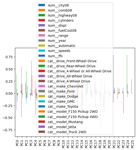
Usually, we will inspect the weights for the first few components. Here, we see .iloc pulling out the first three rows!
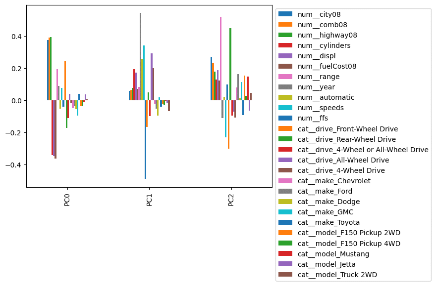
This is still a little hard to interpret because many columns are included that clutter the plot and make it hard to interpret. Let’s limit the components and move the index to the side. (Here’s where Pandas iloc enters the example!)
(comps
 .iloc[:3]
 .plot.bar()
 .legend(bbox_to_anchor=(1,1))
)
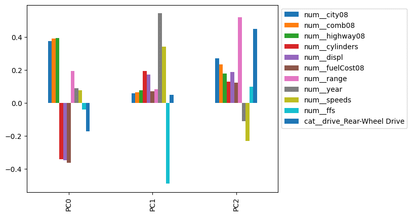
Let's limit the plot only to show columns whose absolute value exceeds some threshold. We combine .pipe with limit_cols to perform this operation:
def limit_cols(df_, limit):
    cols = (df_
            .abs()
            .gt(limit)
            .any()
            .pipe(lambda s: s[s].index)
           )
    return df_.loc[:, cols]

(comps
 .iloc[:3]
 .pipe(limit_cols, limit=.32)
 .plot.bar()
 .legend(bbox_to_anchor=(1,1))
)
This looks much better. It appears that PC0 is impacted most by the city, combined, and highway mileage. PC1 looks like a proxy for year. PC2 is impacted by range, indicating the division between vehicles with electric and combustion engines.
This was an extended example, but probably the most common use I see of .iloc: Pulling off the first (or last) few rows.
My preference would be to rewrite the code without Pandas iloc, like this:
def limit_cols(df_, limit):
    cols = (df_
            .abs()
            .gt(limit)
            .any()
            .pipe(lambda s: s[s].index)
           )
    return df_.loc[:, cols]

num_components = 3

(comps
 #.iloc[:3]
 .head(num_components)
 .pipe(limit_cols, limit=.32)
 .plot.bar()
 .legend(bbox_to_anchor=(1,1))
)
Part 4: Using Pandas Iloc to Index with a Boolean Array
This is a weird one. Generally, when we speak of boolean arrays with Pandas, we refer to a series with the same index as the dataframe (or series) we are working with but with boolean (true / false) values.
Here is a boolean array of vehicles with city mileage above 60:
df.city08 > 600 False
1 False
2 False
3 False
4 False
...
41139 False
41140 False
41141 False
41142 False
41143 False
Name: city08, Length: 41144, dtype: boolLet's see if we can use this boolean array to select the rows of cars with city mileage above 60 in combination with .iloc:
df.iloc[df.city08 > 60]This doesn’t work in Pandas — We get a NotImplementedError:
NotImplementedError: iLocation based boolean indexing on an integer type is not availableIn this case, the term boolean array (for the .iloc docstring) means a list (or NumPy array) with the same length as the number of rows in the dataframe. I'll convert the boolean array to a Python list and try the code again:
df.iloc[list(df.city08 > 60)] barrels08 barrelsA08 charge120 charge240 city08 city08U cityA08 cityA08U cityCD cityE ... mfrCode c240Dscr charge240b c240bDscr createdOn modifiedOn startStop phevCity phevHwy phevComb
7138 0.240 0.0 0.0 0.0 81 0.0000 0 0.0 0.0 41.0000 ... NaN NaN 0.0 NaN Tue Jan 01 00:00:00 EST 2013 Thu Jul 07 00:00:00 EDT 2016 N 0 0 0
7139 0.282 0.0 0.0 0.0 81 0.0000 0 0.0 0.0 41.0000 ... NaN NaN 0.0 NaN Tue Jan 01 00:00:00 EST 2013 Thu Jul 07 00:00:00 EDT 2016 N 0 0 0
8143 0.282 0.0 0.0 0.0 81 0.0000 0 0.0 0.0 41.0000 ... NaN NaN 0.0 NaN Tue Jan 01 00:00:00 EST 2013 Thu Jul 07 00:00:00 EDT 2016 N 0 0 0
8144 0.312 0.0 0.0 0.0 74 0.0000 0 0.0 0.0 46.0000 ... NaN NaN 0.0 NaN Tue Jan 01 00:00:00 EST 2013 Thu Jul 07 00:00:00 EDT 2016 N 0 0 0
8147 0.270 0.0 0.0 0.0 84 0.0000 0 0.0 0.0 40.0000 ... NaN NaN 0.0 NaN Tue Jan 01 00:00:00 EST 2013 Thu Jul 07 00:00:00 EDT 2016 N 0 0 0
... ... ... ... ... ... ... ... ... ... ... ... ... ... ... ... ... ... ... ... ... ...
34563 0.156 0.0 0.0 8.5 138 138.1100 0 0.0 0.0 24.4045 ... TSL standard charger 0.0 80 amp dual charger Thu May 02 00:00:00 EDT 2019 Thu May 02 00:00:00 EDT 2019 N 0 0 0
34564 0.150 0.0 0.0 9.5 140 140.4200 0 0.0 0.0 24.0030 ... TSL standard charger 0.0 80 amp dual charger Thu May 02 00:00:00 EDT 2019 Tue Jun 04 00:00:00 EDT 2019 N 0 0 0
34565 0.180 0.0 0.0 12.0 115 114.9369 0 0.0 0.0 29.3248 ... TSL standard charger 8.0 72 amp dual charger Thu May 02 00:00:00 EDT 2019 Tue Jun 04 00:00:00 EDT 2019 N 0 0 0
34566 0.192 0.0 0.0 12.0 104 104.2314 0 0.0 0.0 32.3367 ... TSL standard charger 8.0 72 amp dual charger Thu May 02 00:00:00 EDT 2019 Tue Jun 04 00:00:00 EDT 2019 N 0 0 0
34567 0.210 0.0 0.0 12.0 98 98.1135 0 0.0 0.0 34.3531 ... TSL standard charger 8.0 72 amp dual charger Thu May 02 00:00:00 EDT 2019 Tue Jun 04 00:00:00 EDT 2019 N 0 0 0
191 rows × 83 columnsThat works! However, I have never found that this felt like the tool to reach for to limit rows of data. I prefer the .query method:
df.query('city08 > 60') barrels08 barrelsA08 charge120 charge240 city08 city08U cityA08 cityA08U cityCD cityE ... mfrCode c240Dscr charge240b c240bDscr createdOn modifiedOn startStop phevCity phevHwy phevComb
7138 0.240 0.0 0.0 0.0 81 0.0000 0 0.0 0.0 41.0000 ... NaN NaN 0.0 NaN Tue Jan 01 00:00:00 EST 2013 Thu Jul 07 00:00:00 EDT 2016 N 0 0 0
7139 0.282 0.0 0.0 0.0 81 0.0000 0 0.0 0.0 41.0000 ... NaN NaN 0.0 NaN Tue Jan 01 00:00:00 EST 2013 Thu Jul 07 00:00:00 EDT 2016 N 0 0 0
8143 0.282 0.0 0.0 0.0 81 0.0000 0 0.0 0.0 41.0000 ... NaN NaN 0.0 NaN Tue Jan 01 00:00:00 EST 2013 Thu Jul 07 00:00:00 EDT 2016 N 0 0 0
8144 0.312 0.0 0.0 0.0 74 0.0000 0 0.0 0.0 46.0000 ... NaN NaN 0.0 NaN Tue Jan 01 00:00:00 EST 2013 Thu Jul 07 00:00:00 EDT 2016 N 0 0 0
8147 0.270 0.0 0.0 0.0 84 0.0000 0 0.0 0.0 40.0000 ... NaN NaN 0.0 NaN Tue Jan 01 00:00:00 EST 2013 Thu Jul 07 00:00:00 EDT 2016 N 0 0 0
... ... ... ... ... ... ... ... ... ... ... ... ... ... ... ... ... ... ... ... ... ...
34563 0.156 0.0 0.0 8.5 138 138.1100 0 0.0 0.0 24.4045 ... TSL standard charger 0.0 80 amp dual charger Thu May 02 00:00:00 EDT 2019 Thu May 02 00:00:00 EDT 2019 N 0 0 0
34564 0.150 0.0 0.0 9.5 140 140.4200 0 0.0 0.0 24.0030 ... TSL standard charger 0.0 80 amp dual charger Thu May 02 00:00:00 EDT 2019 Tue Jun 04 00:00:00 EDT 2019 N 0 0 0
34565 0.180 0.0 0.0 12.0 115 114.9369 0 0.0 0.0 29.3248 ... TSL standard charger 8.0 72 amp dual charger Thu May 02 00:00:00 EDT 2019 Tue Jun 04 00:00:00 EDT 2019 N 0 0 0
34566 0.192 0.0 0.0 12.0 104 104.2314 0 0.0 0.0 32.3367 ... TSL standard charger 8.0 72 amp dual charger Thu May 02 00:00:00 EDT 2019 Tue Jun 04 00:00:00 EDT 2019 N 0 0 0
34567 0.210 0.0 0.0 12.0 98 98.1135 0 0.0 0.0 34.3531 ... TSL standard charger 8.0 72 amp dual charger Thu May 02 00:00:00 EDT 2019 Tue Jun 04 00:00:00 EDT 2019 N 0 0 0
191 rows × 83 columnsPart 5: Using Pandas Iloc to Index with a Callable Function
Here’s another option: passing in a function. You can pass in a function to the index operation or a function for the row selector and/or the column selector. This function should return a single position, a slice, a list, or a tuple of those.
This is very rare in the wild. Here's an example I found: Finding peaks. I'm going to use the find_peaks function from the SciPy library.
The find_peaks function works with NumPy arrays and Pandas series and returns the index locations where the values are above the neighbors that surround them. (You can customize the behavior to constrain the definition of a "peak" as well. We'll use the out-of-the-box behavior.)
from scipy.signal import find_peaksfind_peaks(price_df.IBM)(array([ 2, 4, 7, 9, 14, 19, 24, 28, 31, 34, 36, 38, 48,
53, 56, 59, 65, 68, 70, 72, 76, 80, 83, 85, 91, 94,
103, 107, 117, 119]),
{})Note the return type of this is a tuple. This won’t work directly with .iloc:
price_df.IBM.iloc[find_peaks]This throws a ValueError. (For the sake of brevity, I won’t share the whole traceback.)
ValueError: setting an array element with a sequence. The requested array has an inhomogeneous shape after 1 dimensions. The detected shape was (2,) + inhomogeneous part.This is a great place to uselambda. Let's uselambdato adapt the result offind_peaks:
price_df.IBM.iloc[lambda ser: find_peaks(ser)[0]]2 138.80
4 137.47
7 138.97
9 140.05
14 142.18
19 138.25
24 131.86
28 133.46
31 132.52
34 135.50
36 134.57
38 133.20
48 128.44
53 123.89
56 123.02
59 124.87
65 127.97
68 130.28
70 130.36
72 129.27
76 126.42
80 124.66
83 124.20
85 125.26
91 121.99
94 122.02
103 128.18
107 129.48
117 137.60
119 138.40
Name: IBM, dtype: float64Ok, that works but what is a real life example? We can use it to highlight peaks in a plot:
import matplotlib.pyplot as plt

def plot_with_highlights(ser):
    ax = ser.plot()
    ser.iloc[lambda ser: find_peaks(ser)[0]].plot(linestyle='',
                                                  marker='o')
    return ser

(price_df
 .IBM
 .pipe(plot_with_highlights)
)
0 137.30
1 138.05
2 138.80
3 136.46
4 137.47
...
119 138.40
120 137.48
121 135.96
122 133.69
123 130.91
Name: IBM, Length: 124, dtype: float64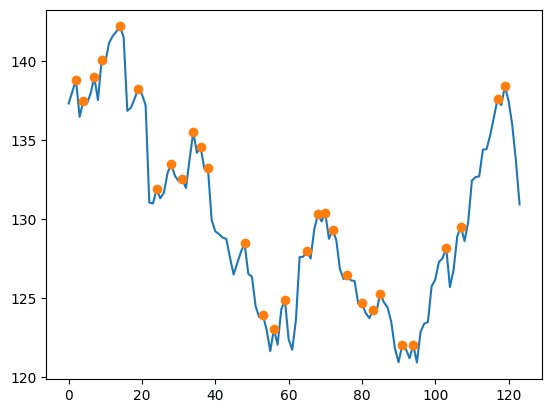
Part 6: Using Pandas Iloc to Index with a Tuple
Finally, the documentation suggests we can also pass in row selectors. We can do this by passing in a tuple. The docstrings states: “A tuple of row and column indexes. The tuple elements consist of one of the above inputs, e.g. (0, 1).”
I'll note that this only applies to dataframes. Using .iloc with series only supports row selectors (because there aren't any columns).
When using .iloc with dataframes, these row selectors can be any of the options we provided above. I have presented some examples of these above.
One thing to note. With .iloc and a dataframe, you can pull out:
- The value of a single cell as a:
- Scalar value
- Column series
- Row Series
- Dataframe
- A Column as a:
- Column series
- Dataframe
- A Row as a
- Row series
- Dataframe
- A subset of a Dataframe
Here is an example of how we can change the types of data results. Looking at our price data, let’s pull out the first BRK-B value. Here’s the whole data:
price_df Date BRK-B DIS F IBM MMM NFLX PG QCOM TSLA UPS ^GSPC
0 2022-12-22 00:00:00-05:00 302.69 86.67 10.51 137.30 118.20 297.75 150.30 109.25 125.35 172.42 3822.39
1 2022-12-23 00:00:00-05:00 306.49 88.01 10.55 138.05 116.79 294.96 150.72 109.41 123.15 173.79 3844.82
2 2022-12-27 00:00:00-05:00 305.55 86.37 10.41 138.80 116.87 284.17 152.04 108.05 109.10 173.72 3829.25
3 2022-12-28 00:00:00-05:00 303.43 84.17 10.17 136.46 115.00 276.88 150.07 105.59 112.71 170.46 3783.22
4 2022-12-29 00:00:00-05:00 309.06 87.18 10.72 137.47 117.21 291.12 150.69 108.42 121.82 172.56 3849.28
... ... ... ... ... ... ... ... ... ... ... ... ...
119 2023-06-15 00:00:00-04:00 339.82 92.94 14.45 138.40 103.81 445.27 148.45 123.61 255.90 179.00 4425.84
120 2023-06-16 00:00:00-04:00 338.31 91.32 14.42 137.48 104.54 431.96 149.54 122.68 260.54 178.58 4409.59
121 2023-06-20 00:00:00-04:00 338.67 89.75 14.22 135.96 102.30 434.70 148.16 119.82 274.45 177.27 4388.71
122 2023-06-21 00:00:00-04:00 338.61 88.64 14.02 133.69 101.47 424.45 149.44 115.76 259.46 173.63 4365.69
123 2023-06-22 00:00:00-04:00 336.91 88.39 14.28 130.91 100.27 420.61 149.79 116.36 261.47 172.37 4368.72
124 rows × 12 columnsHere is a scalar result of the value we want:
price_df.iloc[0, 1]302.69We can pull this out as a column. Note that the index stays the same as the original data, and the series has the column name:
# a column (Series)
price_df.iloc[[0], 1]
0 302.69
Name: BRK-B, dtype: float64Here is the value pulled out as a row. Because Pandas doesn’t have a row type, it changes the row to a series. The column name moves to the index, and the index value moves to the name of the series.
# a row (converted to a Series)
price_df.iloc[0, [1]]
BRK-B 302.69
Name: 0, dtype: objectFinally, we can get the result as a dataframe.
# A Dataframe
price_df.iloc[[0], [1]]
BRK-B
0 302.69What type of value should you pull out of your data? It depends on what you are doing. I find that when I work with row selectors, generally I want dataframes out. When I'm using the .assign method, I generally want a column (series) as a result.
Code Readability and the Danger of Magic Numbers
I’m a huge proponent of writing code that is easy to read, reuse, and share with others. If I have to choose between “easy to write” and “easy to read” code, I will choose easy-to-read every time! In fact, I will often write more code to make it easier to read.
So let’s talk about something that is easy to write, but often makes code hard to read, and comes up a lot when people use Pandas iloc: magic numbers.
In the world of programming, magic numbers refer to literal numbers that appear directly in the source code without any explanation. They are “magic” in that they “just work.” Over time, it becomes harder and harder for you (and certainly for your colleagues) to understand why these specific numbers were chosen, which can lead to errors and difficulties when updating or modifying the code.
For instance, consider the following:
selected_data = sales_data.iloc[0:5, 2:4]In this case, 0, 5, 2, and 4 are magic numbers. Did you want the first five rows? Are those five rows specific to data at a particular time? If you run the code later, will the rows be in the same location? Similarly, with the columns? Did you just want the third and fourth column? What if more columns are added? This code might work, but the intent is not clear.
One of the most effective ways to avoid magic numbers is to use meaningful variable names instead. For example, instead of directly using numbers with .iloc, we could define variables that describe what these numbers represent:
start_row = 0
end_row = 5
start_column = 2
end_column = 4
selected_data = sales_data.iloc[start_row:end_row, start_column:end_column]
In this case, we’ve replaced the magic numbers 0 and 5 with the variables ‘start_row’ and ‘end_row’. This makes the code much more understandable: it’s clear that we’re selecting the rows from ‘start_row’ to ‘end_row’.
But my preference, if we wanted the first five rows and two specific columns, would be to avoid Pandas iloc entirely:
num_rows = 5
(sales_data
  .head(num_rows)
  .loc[:, ['Country', 'Sales_Amount']]
)
Although this requires more typing, this code makes our intent clear. When doing quick and dirty analysis, I might use the .iloc version, but when I start working with others, I will refactor.
Conclusion
Thanks for reading part two of our ultimate guide to indexing in Pandas. You should now be aware of some of the capabilities of.iloc, which lets you pull out rows or columns based on integer location. This property is handy, but it is usually possible (and preferable) to refactor.ilocout of our code.
If you liked this, check out our previous Professional Pandas posts on Pandas loc, the Pandas merge method, and the Pandas assign method / chaining.
About Ponder
Ponder is the company that lets you run your Python data workflows (in Pandas or NumPy) securely, seamlessly, and scalably in your data warehouse or database. Sign up for a free trial!
Try Ponder Today
Start running your Python data science workflows in your database within minutes!